ARMA Modeling

The ARMA model is the most general, so we treat it first. An ARMA model is a combination of an AR model and an MA model. We can create ARMA data by a cascade of two recursions. Let the intermediate AR sequence $y_t$ be created according to

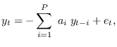$$y_t = -\sum_{i=1}^P \; a_i \;y_{t-i} + e_t,$$ (10.12)

where the sequence $e_t$ are iid Gaussian RV with variance $\sigma^2$. This is followed by an MA recusion to generate $x_t$:

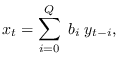$$x_t = \sum_{i=0}^Q \; b_i \; y_{t-i},$$ (10.13)

where we let $b_0=a_0=1$. Refer to Kay [31] for a full description. In MATLAB, an ARMA process can be generated with the filter command:

>> e=randn(N,1);
>> x=filter(b,a,e * sqrt(sig2));

which is directly equivalent to (10.12),(10.13) except for the initial startup. To alleviate startup effects, it is necessary to discard the initial samples of x. The number of samples to discard is related to how fast $r_t$ decays to zero. Let that be $L$ samples. In practice, one would generate $N+L$ samples, then keep the last $N$ samples:

>> e=randn(N+L,1);
>> x=filter(b,a,e * sqrt(sig2));
>> x=x(L+1:L+N);