CR Bound analysis of ARMA PDF - exact forms.

The results in this section are used in the function software/pdf_arma_exact.m. We now find the derivatives of (10.6) with respect to the parameters ${\bf b}, {\bf a},\sigma^2$. In MATLAB, we write (10.6) as

  R=toeplitz(r(1:N));
  lpx = -N/2*log(2*pi)-.5*log(det(R)) - .5*x'*inv(R)*x);

We note that the derivative of lpx with respect to a scalar parameter $\theta$ is

  Ri=inv(R);
  lpx_theta = -.5*trace( Ri * D )  + .5 * x'*Ri*D*Ri*x;

where D is $N$-by-$N$ matrix of derivatives of the elements of R with respect to $\theta$. It makes use of the fact that R is symmetric (otherwise it would be -.5*trace( Ri' * D ) + .5 * x'*Ri'*D*Ri*x). Since R is formed from R=toeplitz(r(1:N));, we can write that D=toeplitz(d(1:N));, where d is $N$-by-$1$ vector of derivatives of the elements of r with respect to $\theta$.

  D=toeplitz(d(1:N));
  lpx_theta = -.5*trace( Ri * D )  + .5 * x'*Ri*D*Ri*x;

We can write r in terms of the ARMA parameters in a simple form if we make use of the fact that for a stable ARMA process, r must eventually decay to zero. For large enough $L$, $r_t \simeq 0$ for $t>L$. Then, we can treat r as a circular ACF, the inverse DFT of a circular power spectrum of size $2L$. Thus, the values of the circular PSD of length $2L$ computed using (10.9) will be the same as the true PSD at discrete frequencies. Therefore, the circular ACF will match the first $L$ values of the true ACF. Let rho be the length-$2L$ circular PSD. If,

  r = real(ifft(rho));

then the first $N$ values of r are the true ACF values. Since d is $N$-by-$1$ vector of derivatives of the elements of r with respect to $\theta$, it follows from the chain rule for derivatives that

  d = real(ifft(rho_theta));

where rho_theta is the vector of derivatives of the elements of rho with respect to parameter theta. These derivatives are

$$\begin{array}{rcl} \left( \frac{\partial \rho_k}{\partial b_m... ...t) & =& \frac{\vert B_k\vert^2}{\vert A_k\vert^2 }. \end{array}$$ (10.22)

In summary,

  d = real(ifft(rho_theta));
  D=toeplitz(d(1:N));
  Ri=inv(R);
  lpx_theta = -.5*trace( Ri * D )  + .5 * x'*Ri*D*Ri*x;

The problem with this approach is the necessity of computing and storing the $N$-by-$N$ matrices R and D. But, using the fact that they are Toeplitz, we can simplify the problem to:

  y = toepsolve(r,x); % y = inv(toeplitz(r)) * x; 
  d = real(ifft(rho_theta));
  D=toeplitz(d(1:N));
  H = toepsolve(r(1:N),D);
  lpx_theta = -.5*trace(H)  + .5 * y'*D*y;

where x=toepsolve(r,b); uses the Levinson algorithm to solve the general symmetric toeplitz system b = toeplitz(r)*x; for x. Note that if B is a matrix, X=toepsolve(r,B); will solve the problem for each column of B in turn. Since we still need to store H and D unecessarily (we need only the trace of H and D is Toeplitz), it makes sense to code up a special function

  function L=toep_special(B,r,y,N);
  % solves the problem:
  %
  %    for i=1:size(B,2),
  %       D=toeplitz(B(1:N,i));
  %       H = inv(R) * D;
  %       L(i) = -.5*trace(H)  + .5 * y'*D*y;
  %    end;
  % where
  %    R = toeplitz(r(1:N));
  %    y = inv(R) * x;
  %
  % for each column of B without having to store R, H,  or D,
  % or take the inverse of a matrix!!!
  % If each column of B is the derivative of the power spectrum
  % with respect to a different parameter, and r is the ACF,
  % and x is the raw data, then the output are the derivatives of the log-PDF
  %    lpx = -N/2*log(2*pi)-.5*log(det(R)) - .5*x'*inv(R)*x);
  % with respect to the parameters

In summary, we can compute the exact derivatives of (10.6) with respect to the ARMA parameters as follows:

    A=fft([a(:); zeros(2*L-P-1,1)]);
    B=fft([b(:); zeros(2*L-Q-1,1)]);
    A2=msq(A);
    B2=msq(B);
    h = B2./A2;
    rho = sig2 * h;
    r = real(ifft(rho));
    E=exp(-1i*2*pi/N/2*[0:2*N-1]' * [0:max(P,Q)]);
    [y,ldetR] = toepsolve(r(1:N),x(1:N),N); % y = R \ x;
    Rho_a =  -2 * sig2 * real( repmat(h./A,1,P) .* E(:,2:P+1) );
    Rho_b =  2 * sig2 * real( repmat(h./B,1,Q) .* E(:,2:Q+1) );
    R_a = real(ifft(Rho_a));
    R_b = real(ifft(Rho_b));
    da = toep_special(R_a(1:N,:),r(1:N),y(1:N),N);
    db = toep_special(R_b(1:N,:),re(1:N),y(1:N),N);

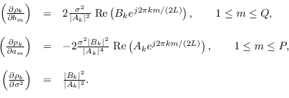
Note that Rho_a be the matrix where column Rho_a(:,m) is rho_theta for parameter $a_{m+1}$ and Rho_b be the matrix where column Rho_b(:,m) is rho_theta for parameter $b_{m+1}$. We can do the same for the scalar paremeter $\sigma^2$:

    rho_sig =  h;
    r_sig = real(ifft(rho_sig));
    dsig = toep_special(r_sig(1:N),r(1:N),y(1:N),N);

however, a more compact form can be shown to be

    dsig = -.5*N/sig2 + .5 * y(1:N)'*x(1:N)/sig2;

The second derivatives may also be obtained and the Fisher's information computed. Let $\theta$, $\phi$ be two general spectral parameters. Then

$$\begin{array}{rcl} {\displaystyle { \partial \log p({\bf x}... ... R}^{-1} {\bf D}^\theta {\bf R}^{-1} {\bf D}^\phi) \end{array}$$

The terms ${\bf H}^\theta = {\bf R}^{-1} {\bf D}^\theta$ and ${\bf H}^\phi = {\bf R}^{-1} {\bf D}^\phi$ can be obtained by

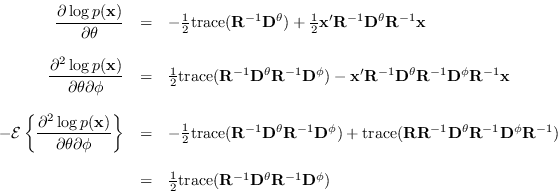
  H_theta = toepsolve(r,D_theta);

We can simplify matters if we notice that for two matrices A, B, we have trace( A * B) is the same as sum( C(:) ) where C= A .* B';. The function toep_fim efficiently computes

  function Q=toep_fim(B,r,L);
  % solves the problem:
  %
  %    R = toeplitz(r);
  %    for i=1:size(B,2),
  %       Di=toeplitz(B(:,i));
  %       for j=1:size(B,2),
  %         Dj=toeplitz(B(:,j));
  %         Q(i,j) = .5*trace(inv(R)*Di*inv(R)*Dj);
  %       end;
  %    end;
  %

See software/pdf_arma_exact.m for details.