Rational Transfer Function Models
In this chapter, we are concerned with rational
transfer function models driven by independent Gaussian noise.
Let  be a sequence of
iid Gaussian noise samples of variance
be a sequence of
iid Gaussian noise samples of variance  .
Squence has a power spectrum (10.1) of
.
Squence has a power spectrum (10.1) of
Linear system theory teaches that the power spectrum at the output
of a linear system is equal to the input power spectrum
times the magnitude-squared of the transfer function.
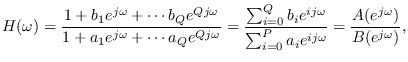
The general form of the rational transfer function is
where we have assumed  ,
,  .
It follows that the power spectrum of
.
It follows that the power spectrum of  is given by
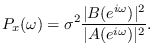 |
(10.8) |
The corresponding length- circularly-stationary process has circular
power spectrum
circularly-stationary process has circular
power spectrum
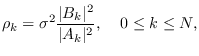 |
(10.9) |
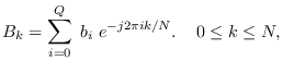
where  and
and  are the length- DFTs of the numerator and denominator coefficient
sequences.
are the length- DFTs of the numerator and denominator coefficient
sequences.
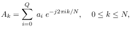 |
(10.10) |
and
 |
(10.11) |
If  and the numerator is 1, the model is said to be
autoregressive (AR).
If
and the numerator is 1, the model is said to be
autoregressive (AR).
If  and the denominator is 1, the model is said to me moving average (MA).
If
and the denominator is 1, the model is said to me moving average (MA).
If  and
and  , this is the form of the autoregressive-moving average (ARMA) model.