CR bound analysis of circular ARMA parameters pdf_arma_circ.m.
The circular ARMA model lends itself better to analysis.
The CR bound for the circular ARMA model parameters
are derived now.
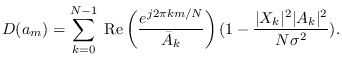
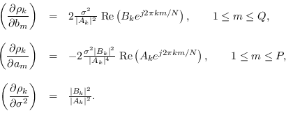
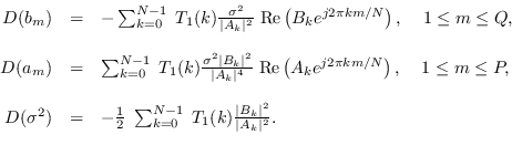
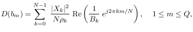
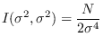
We analyze the PDF (10.18) for the CR bound.
We apply the results of Section 17.2.2 with
 |
(10.23) |
noting that the ARMA parameters are spectral parameter  .
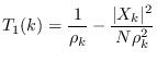
Following these results, we need the derivatives of the spectral values
.
Following these results, we need the derivatives of the spectral values  with respect to
the parameters. The first derivatives are
(from eq. 10.22 with
with respect to
the parameters. The first derivatives are
(from eq. 10.22 with  replaced by
  ).
).
 |
(10.24) |
Thus,
 |
(10.25) |
where
 |
(10.26) |
We can simplify (10.25). For example, we can rewrite  as
as
The  in the last term can be ignored since
because
 is the DFT of an anti-causal sequence. This leaves
 |
(10.27) |
Similarly,
 |
(10.28) |
Using (10.24), (17.9),
 |
(10.29) |
and
 |
(10.30) |
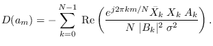
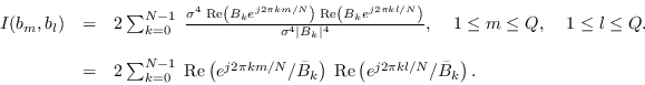
A simple form for
 can be found. We re-write (10.30) as
 |
(10.31) |
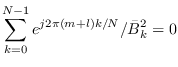
Note that the frequency-domain function
is the DFT of an anti-causal function since both  and
and  are causal, so
for
 giving
 |
(10.32) |
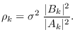
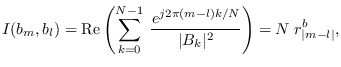
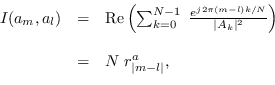
where  is the ACF of the
  -th order AR process with parameters
   rb = rlevinson(b,1);
   Ibb = toeplitz(rb(1:Q)) * N;
Similarly,
 |
(10.33) |
which is the same form as (10.30), so we can copy the form of (10.32) to arrive at
 |
(10.34) |
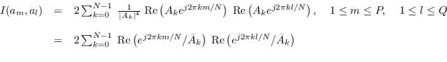
where  is the ACF of the
  -th order AR process with parameters
   ra = rlevinson(a,1);
   Iaa = toeplitz(ra(1:P)) * N;
Also,
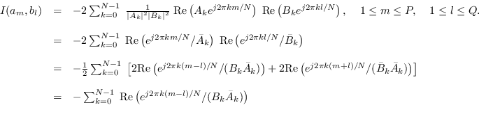 |
(10.35) |
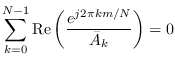
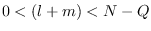
We also arrive at
because  is zero for negative
  .
Similarly,
.
Similarly,
(See [31] p. 277 for additional information).
A MATLAB implementation for
 ,
,
 ,
is
provided below (See
software/pdf_arma_circ.m).
,
is
provided below (See
software/pdf_arma_circ.m).
>>   A=fft([a(:); zeros(N-P-1,1)]);
>>   B=fft([b(:); zeros(N-Q-1,1)]);
>>   E=exp(-1i*2*pi/N*[0:N-1]' * [0:max(P,Q)]);
>>   Hb = real( E(:,2:Q+1) .* repmat(1./B,1,Q) );
>>   Ha = real( E(:,2:P+1) .* repmat(-1./A,1,P) );
>>   I.a_a = 2 * Ha' * Ha;
>>   I.a_b = 2 * Ha' * Hb;
>>   I.b_b = 2 * Hb' * Hb;