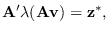
Note that (7.8) is equivalent to the statement
that the vector
 is in the column space of
  ,
or that there exists a free variable
,
or that there exists a free variable  such that
As an aside, note that condition (7.8) also assures that (7.5)
will have zero derivative along the manifold, which is one of
the assumptions of the surrogate density.
The method to find the centroid is to find the
vector such that
 |
(7.10) |
where

 is equation (7.3) applied element-wise.
This is essentially the same as for the
positive-
is equation (7.3) applied element-wise.
This is essentially the same as for the
positive- case (5.18) , except that the non-linear relationship
between
case (5.18) , except that the non-linear relationship
between
 and
is different.
The algorithm of Section
5.3.2 to find
based on
driving (5.20) to zero can be used if
and
is different.
The algorithm of Section
5.3.2 to find
based on
driving (5.20) to zero can be used if
 and
the diagonal elements of
and
the diagonal elements of
 in (5.21)
are given by
in (5.21)
are given by
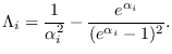 |
(7.11) |
Let
 be the value of
at the solution to (7.10).
The modified algorithm to find
is:
be the value of
at the solution to (7.10).
The modified algorithm to find
is:
- Set iteration counter
 .
.
- To initialize, let
.
-
 . Initially,
will be the
vector of zeros.
. Initially,
will be the
vector of zeros.
- Compute
 from
using (7.3) element-wise.
from
using (7.3) element-wise.
- Compute derivative and Hessian according to (5.21) and (5.23),
and (7.11), then update :
- Increment
 and go to step 3.
The above algorithm is implemented by software/lam_solve.m with dbound=1.
![$\displaystyle {\bf v}_{n+1} = {\bf v}_n +
\left[ \frac{\partial^2 \rho}{\partial u_k \partial u_l}\right]^{-1}
\left[ \frac{\partial \rho}{\partial u_k}\right].$](img687.png)