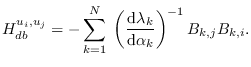
To compute the Hessian, we take the derivative of (7.7) with respect to  ,
,
 |
(7.9) |
The following algorithm is proposed
- Determine the pseudo-inverse solution
 (5.11).
- Seek an initial starting point for

 , a vector that meets (5.12)
and has elements on
, a vector that meets (5.12)
and has elements on ![$[0,1]$](img9.png) .
Use an off-the-shelf linear programming solver as
explained in Section 5.3.1.
.
Use an off-the-shelf linear programming solver as
explained in Section 5.3.1.
- Compute free variable
 so that
 using
using
 .
.
- Determine
 from
by solving (7.3) for
from
by solving (7.3) for  , for each
  .
.
- Compute entropy (7.6) and first and second derivatives (7.7),(7.9).
- Take a Newton-Raphson iteration :
where
 and
and
 are the Hessian and gradient
of
are the Hessian and gradient
of  with respect to
  .
.
- Re-compute the mean :
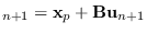 . Check that
all elements of
. Check that
all elements of
 are in .
If not, take a smaller step.
are in .
If not, take a smaller step.
- Go to step 4.
The above algorithm is implemented by software/me_lin_01.m.