Starting point

As we mentioned, we need to start MCMC-UMS with a valid ${\bf x}$. Inversion of the dimension-reducing transformation ${\bf z}={\bf A}^\prime {\bf x}$ using pseudo-inverse

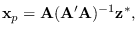$${\bf x}_p = {\bf A}({\bf A}^\prime {\bf A})^{-1} {\bf z}^*,$$ (5.11)

produces a solution for ${\bf x}$ that meets the linear constraint ${\bf A}^\prime {\bf x}= {\bf z}^*$, but may have negative-valued elements. A good initial starting point can be obtained from any linear-programming solver. Specifically, we find the solution to the maximization of $q=\sum_{i=1}^N x_i$ subject to ${\bf x}\in {\cal M}({\bf z}^*).$ It makes no difference if we are maximizing or minimizing since $q$ is fixed anyway by the linear constraints. Any linear programming (LP) algorithm such as OCTAVE glpk.m or MATLAB linprog.m can output a “solution" which is a valid point. See software/module_A_chisq_synth for additional details. The best starting point, however, is the manifold centroid, discused in Section 5.3.2.