Predicting the Mean (centroid) of MCMC-UMS.

For convex manifolds, the manifold centroid $\bar{{\bf x}}_z$ is the center of mass in Figure 5.8 and is on the manifold. It is also the conditional mean ${\cal E}({\bf x}\vert{\bf z}^*)$, and is an optimal point with respect to a deterministic entropy measure. It has applications in feature inversion, image reconstruction and spectral estimation.

The centroid can be approximated by the sample mean of samples generated using UMS, or much more efficiently using the “surrogate density" approach, which we now explain. Let $p_s({\bf x})$, be a PDF with support on ${\cal X}$ (not limited to the manifold), but sharing four properties with $\mu({\bf x}\vert{\bf z}^*; T)$: (a) its mean $\lambda$ lies on the manifold, so

$${\bf A}^\prime \lambda={\bf z}^*, \;\;\;\; {\rm such \; that\;} \bar{x}_i>0, \; {\rm for \; all}\; i,$$ (5.12)

(b) it has constant density along the manifold (meaning that the gradient in a direction aligned with the manifold is zero), (c) it has maximum possible entropy under the constraint (5.12), and (d) it has support in all of ${\cal X}$, but itsprobability mass is concentrated near the manifold. This idea is illustrated in Figure 5.9. The property that the samples congregate near the manifold for $N$ large can be justified by the law of large numbers (See Appendix in [24]). As a result, the surrogate density converges effectively to the manifold distribution. Therefore, the mean $\lambda$ of the surrogate density is a very good approximation to the manifold centroid $\bar{{\bf x}}_z$ at high dimensions.

Figure: Illustration of surrogate density. An arbitrary sample ${\bf x}$ is decomposed into a component ${\bf x}_A$ in the column space of ${\bf A}$ and the orthogonal component ${\bf x}_B$. At high dimension, samples congregate near the manifold where ${\bf A}^\prime {\bf x}= {\bf z}$ and are equally distributed along the manifold.

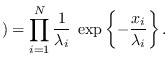
The property that the surrogate distribution is uniform along the manifold can be seen once we select the surrogate density and maximize its entropy. It is known that the exponential density has the highest entropy among all densities for positive-valued ${\bf x}$ with specified mean $\lambda$ [39].

$$p({\bf x}; \mbox{\boldmath$\lambda$} ) = \prod_{i=1}^N \frac{1}{\lambda_i} \; \exp\left\{ -\frac{x_i}{ \lambda_i}\right\}.$$ (5.13)

We therefore propose to use (5.13) as the surrogate density for $\mu({\bf x}\vert{\bf z}^*; T)$, by maximizing the entropy of (5.13) over $\lambda$, subject to ${\bf A}^\prime$   $\lambda$$={\bf z}^*.$ The entropy of (5.13) is

$$Q_p=\sum_{i=1}^N (1+\log \lambda_i),$$ (5.14)

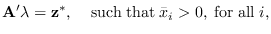
where “p" indicates positive data case. If we use (5.10) to write $\lambda$ in terms of ${\bf u}$, we can maximize $Q_p$ over ${\bf u}$. The solution must meet the requirement that the derivatives of the entropy with respect to $u_k$ are zero, or

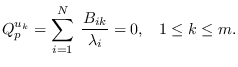$$Q_p^{u_k} = \sum_{i=1}^N\; \frac{B_{ik}}{\lambda_i} = 0,\;\;\; 1\leq k \leq m.$$ (5.15)

This condition forces the distribution to be constant on the manifold. To see this, first, let ${\bf x}$ be decomposed as (See Figure 5.9), ${\bf x}={{\bf x}}_A + {\bf B}{\bf u}$, where matrix ${\bf B}$ spans the subspace orthogonal to matrix ${\bf A}$. Note that changes to vector ${\bf u}$ will move ${\bf x}$ within the manifold, but not change its projection onto the columns of ${\bf A}$, so ${\bf x}$ remains on the manifold. Therefore, a distribution is constant on the manifold if and only if its derivative w/r to ${\bf u}$ is zero. It is easily shown that the derivative of $\log p({\bf x};$$\lambda$$)$ with respect to $u_k$ equals $-\sum_{i=1}^N \frac{B_{i,k}}{ \lambda_i}$, making (5.15) equivalent to requiring $p({\bf x};$$\lambda$$)$ to be constant on the manifold.

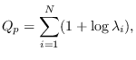
Incidentally, note that maximizing (5.14) also maximizes the classical maximum entropy measure

$$H_s({\bf x}) = \sum_{i=1}^N \; \log x_i,$$ (5.16)

which is used in classical spectral estimation [40,41] and image reconstruction [42,43].

There are two ways to solve (5.15), one requiring a valid starting point in the manifold, and one not requiring a starting point.