Data re-synthesis of positive data from linear features: UMS
We now turn our attention to the re-synthesis of  from
from  using UMS.
This function is implemented by software/module_A_chisq_synth.m.
The theory behind the method is not simple, and deserves
a lengthy treatment.
using UMS.
This function is implemented by software/module_A_chisq_synth.m.
The theory behind the method is not simple, and deserves
a lengthy treatment.
Given a fixed feature, say  , we sample from the manifold
 |
(5.9) |
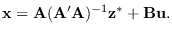
In general, we can access the desired manifold by
using the linear space orthogonal to
the columns of  .
Let matrix
.
Let matrix  defined as in Section 4.4.
Let
defined as in Section 4.4.
Let
 |
(5.10) |
Thus,  is the ancillary statistic
that spans the manifold.
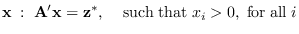
We need to generate samples uniformly in
within the region that meets the positivity constraint
in (5.9).
Uniformly sampling in creates a uniformly-sampled
region in , but unfortunately, it is difficult to find the region
in
is the ancillary statistic
that spans the manifold.
We need to generate samples uniformly in
within the region that meets the positivity constraint
in (5.9).
Uniformly sampling in creates a uniformly-sampled
region in , but unfortunately, it is difficult to find the region
in
 which maps to
 .
Rejection sampling is known to suffer from exponentially
decreasing acceptance rate.
A method based on Hit-and-Run sampling, described in Section
5.3.1, can efficiently generate
samples uniformly distributed on the manifold.
.
Rejection sampling is known to suffer from exponentially
decreasing acceptance rate.
A method based on Hit-and-Run sampling, described in Section
5.3.1, can efficiently generate
samples uniformly distributed on the manifold.
To visualize the distribution of generated using UMS, we
conducted the following experiment.
We used a feature of dimension  , with the first feature
equal to
, with the first feature
equal to
 , and generated random samples of
on the manifold using rejection sampling.
Figure 5.7 (top left) shows samples of
, and generated random samples of
on the manifold using rejection sampling.
Figure 5.7 (top left) shows samples of  showing the
desired uniform distribution.
Figure 5.7 (top right) shows the histogram of
showing the
desired uniform distribution.
Figure 5.7 (top right) shows the histogram of  for 10000 samples.
Figure:
From top: manifold sampling results for  ,
,
 , and
, and  (manifold dimension 2,4,8, respectively).
Left: random samples of
(manifold dimension 2,4,8, respectively).
Left: random samples of  , . Right,
histogram of .
, . Right,
histogram of .
|
|
For manifold dimensions above 2, the manifold distribution
does not look uniform when projected onto a 2D plane
even though it is uniform in the higher dimensions. With increasing
manifold dimension, the histogram on the right side of the figure looks
increasingly exponential. This effect is analogous to Figure 4.1,
which tended to Gaussian. There is an analogous argument
based on the fact that dividing a set of exponential random variables
by their sum, generates uniform distribution
on a simplex [26] (the constraint that
is fixed constrains
to a simplex).
Subsections
![\includegraphics[height=1.5in,width=4.0in]{x1x2exphist4.eps}](img616.png)
![\includegraphics[height=1.5in,width=4.0in]{x1x2exphist6.eps}](img617.png)
![\includegraphics[height=1.5in,width=4.0in]{x1x2exphist10.eps}](img618.png)