Asymptotic (large $N$) behavior

To visualize the sampling distribution, we can generate random samples on the manifold for a fixed feature value, and plot the pair $(x_l, x_m)$ for two indexes $l,m$ on a plane. For a simple example, we let the feature be the two statistics 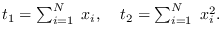$t_1= \sum_{i=1}^N \; x_i, \;\;\;\; t_2= \sum_{i=1}^N \; x_i^2.$ Therefore, ${\bf A}=[1,\; 1, \; \ldots 1]^\prime,$ and $D=1$. Figure 4.1 shows a simulation for $N=3,4,$ and $64$. The initial feature value ${\bf z}$ was created by drawing a random ${\bf x}\in{\cal R}^N$ from a standard normal distribution, and computing $t_1,t_2$. With $nbfz$ fixed, we generated random samples of ${\bf x}$ on the manifold. On the left, we see random samples of ${\bf x}$ plotted on the $x_1,x_2$ plane. On the right, we see a histogram of $x_2$. Interestingly, for a 2-dimensional manifold, $N-D=2$, the samples will fall on an elliptical curve. One can see that with increasing manifold dimension, the marginal distributions approach Gaussian, even though the sampling is uniform on the manifold. This can be understood since it is well known that normalizing a vector of independent Gaussian random variables by its 2-norm generates points uniformly distributed on a hyper-sphere [26]. Since the normalization constant converges to a constant at high dimension, it follows that the distribution of ${\bf u}$ is approximately Gaussian.

Figure: From top, manifold sampling results for $N=3$, $N=4$, and $N=64$. Left: random samples of $x_1$, $x_2$. Right, histogram of $x_2$.