Whitened MCMC-UMS
We may improve mixing even further by “whitening" the
problem.
Since we have verified that
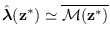 ,
we can now predict the mean of the MCMC-UMS procedure
and can transform the problem.
Let
,
we can now predict the mean of the MCMC-UMS procedure
and can transform the problem.
Let
 be the “whitened" raw input spectrum,
and
 the compensated matrix
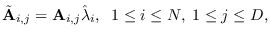 which obtains the same feature
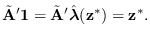
The new linear constraint “manifold" is:
 |
(5.25) |
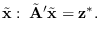
As a starting vector for
, we can use the
vector of ones, denoted by  , since clearly
 The MCMC-UMS procedure, then should produce random spectral vectors
that have approximate mean and meet (5.25).
These random vectors can be transformed
to produce solutions to the original problem
The MCMC-UMS procedure, then should produce random spectral vectors
that have approximate mean and meet (5.25).
These random vectors can be transformed
to produce solutions to the original problem
The vectors produced this way are actually
random samples for the original problem
because they are in
 and the linear whitening operation preserves the uniform distribution.
The result of whitening can be seen in Figure 5.12
and the result is dramatic. The change in ESS
(seen by drawing a horizontal line)
and is more than an order of magnitude
for both systematic and random directions.
and the linear whitening operation preserves the uniform distribution.
The result of whitening can be seen in Figure 5.12
and the result is dramatic. The change in ESS
(seen by drawing a horizontal line)
and is more than an order of magnitude
for both systematic and random directions.