ML approach
Under certain conditions, the J-function is independent of  as long
as remains within the “region of sufficiency" (ROS) for
as long
as remains within the “region of sufficiency" (ROS) for  (See Section 2.3.3).
Then, can even “float" with the data
as long as it remains in the ROS.
The ROS can be spanned by a parametric model
(See Section 2.3.3).
Then, can even “float" with the data
as long as it remains in the ROS.
The ROS can be spanned by a parametric model
 as long as (a)
 for some parameter
  , and (b)
is a sufficient statistic for
, and (b)
is a sufficient statistic for  .
.
We can easily meet these conditions using
the multi-variate TED distribution (7.5) with

 .
Condition (a) is met by
.
Condition (a) is met by
 . Condition (b)
is met since (7.5) can be written
. Condition (b)
is met since (7.5) can be written
 for some function
  . It therefore follows that
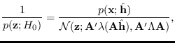
 |
(17.16) |
for any , where
 is defined as the
distribution of when
is defined as the
distribution of when
 .
Since the ratio (17.16) does not depend on
, it makes sense to place at the
point where
can be easily evaluated,
and that is the point where both
and
have their maximum value, that is to say
at the maximum likelihood (ML) point
.
Since the ratio (17.16) does not depend on
, it makes sense to place at the
point where
can be easily evaluated,
and that is the point where both
and
have their maximum value, that is to say
at the maximum likelihood (ML) point
At this point, we can apply the central limit theorem
to find
 . The mean is given by
where
 is expected value,
and
is expected value,
and
 is the TED mean (7.3).
Note that under
is the TED mean (7.3).
Note that under
 ,
,
where
[97,98].
From this, we can solve for the variance of  ,
,
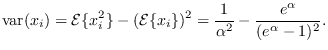 |
(17.17) |
The covariance of is therefore
where  is the diagonal matrix with elements (17.17).
Finally, then, we apply (17.16) at
is the diagonal matrix with elements (17.17).
Finally, then, we apply (17.16) at
 ,
and
,
and
 , to get
 |
(17.18) |
where


 is the Gaussian distribution
with mean
and covariance
is the Gaussian distribution
with mean
and covariance  .
This approach can then be compared numerically with the
reciprocal of (2.12).
.
This approach can then be compared numerically with the
reciprocal of (2.12).
![$\displaystyle {\cal E}\{x_i^2\} =
\frac{2}{\alpha^2}
\left[
\frac{1-\frac{1}{2} \left( \alpha^2 -2\alpha + 2\right) e^\alpha}{1-e^\alpha}
\right],$](img1966.png)