Numerical validation

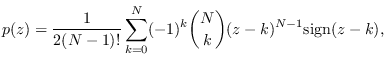
We now compare the methods of Sections 17.7.1 and 17.7.2 for a special case where $p({\bf z})$ can be computed exactly. Consider the trivial case where ${\bf A}=[1, \; 1, \ldots 1]^\prime$. In this case ${\bf z}={\bf A}^\prime {\bf x}$ has the Irwin-Hall distribution

$$p(z) = \frac{1}{2(N-1)!} \sum_{k=0}^N(-1)^k \binom Nk (z-k)^{N-1} {\rm sign}(z-k),$$

where ${\rm sign}(0)=0.$ In Figure 17.1, we show the $\log p({\bf z})$ error (compared with exact Irwin-Hall distribution) on the Y-axis for both methods for $N=10$ and $N=40$. The error is very small, less that .02 at $N=10$ and less than .004 at $N=40$. This error for a 40-dimensional PDF is very small and for all practical purposes, can be ignored. Notice that the error becomes smaller with increasing $N$. For even larger $N$, however, the round-off error in computing Irwin-Hall eventually dominates. Although almost always the same, the ML approach had slightly more error and the SPA was faster. Therefore, SPA is our method of choice.

Figure: Numerical comparison of SPA (dots) and ML (circles) with Irwin-Hall distribution (X-axis) for $N=10$ and $N=40$.