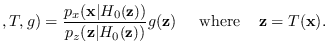
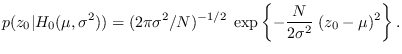
Floating Reference Hypothesis

One way to alleviate potential numerical issues in evaluating $p({\bf z}\vert H_0)$ and/or $p({\bf x}\vert H_0)$, is with a floating reference hypothesis. Under certain conditions, the reference hypothesis $H_0$ may be changed “on the fly" to alleviate numerical or PDF approximation issues with the calculation of the J-function. Loosely stated, $H_0$ is allowed to vary within a set of hypotheses that can be optimally distinguished using the feature ${\bf z}$. For example, as long as ${\bf z}$ contains the sample variance, which is a sufficient statistic for distinguishing two zero-mean Gaussian densities that differ only in variance, then $H_0$ may be the zero-mean Gaussian distribution with arbitrary variance - as the assumed variance varies, the numerator and denominator terms of the J-function vary over a wide range, but the ratio (the J-function) remains constant. Therefore, for numerical convenience, we can set the variance to the value at or near the maximum of both the numerator and denominator.

We first define the region of sufficiency (ROS) of feature set transformation ${\bf z}=T({\bf x})$, denoted by ${\cal H}_z$, as a set of hypotheses such that every pair of hypotheses $H_{0a}, H_{0b}\in {\cal H}_z$ obeys the relationship

$${p_x({\bf x}\vert H_{0a})\over p_x({\bf x}\vert H_{0b})}= {p_z({\bf z}\vert H_{0a})\over p_z({\bf z}\vert H_{0b})}.$$

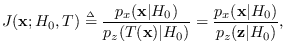
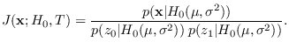
Thus, a likelihood ratio between any two hypotheses in ${\cal H}_z$ can be optimally constructed either in the raw data or in the feature space without loss of information. An ROS may be thought of as a family of PDFs traced out by the parameters of a PDF where ${\bf z}$ is a sufficient statistic for the parameters. We can re-arrange the above equation as follows:

$${p_x({\bf x}\vert H_{0a})\over p_z({\bf z}\vert H_{0a})}= {p_x({\bf x}\vert H_{0b})\over p_z({\bf z}\vert H_{0b})}.$$

Thus, the “J-function",

$$J({\bf x};H_0,T) \stackrel{\mbox{\tiny$\Delta$}}{=} {p_x({\bf x}\... ..._z(T({\bf x})\vert H_0)} = {p_x({\bf x}\vert H_0) \over p_z({\bf z}\vert H_0)},$$ (2.13)

is independent of $H_0$ as long as $H_0$ remains within ROS ${\cal H}_z$.

Defining the ROS should in no way be interpreted as a sufficiency requirement for ${\bf z}$. Every feature has a ROS, because at the very least, the projected PDF itself (2.2) serves a one hypothesis, and $H_0$ as another, for which the feature is sufficient. As long as the feature contains an energy statistic (see Section 3.2.2), the J-function is independent of scale parameters in $H_0$.

Example 3   We re-visit example 1 with an eye to using a floating reference hypothesis. Let $H_0(\mu, \sigma^2)$ be the hypothesis that ${\bf x}$ is a set of $N$ independent identically distributed Gaussian samples with mean $\mu$ and variance $\sigma^2$. We now show that ${\bf z}$ is a sufficient statistic for $(\mu, \; \sigma^2)$, and an ROS for ${\bf z}$ is the set of all PDFs traced out by $(\mu, \; \sigma^2)$. We have

$$p({\bf x}\vert H_0(\mu,\sigma^2)) = (2\pi\sigma^2)^{-N/2} \; \exp\left\{ -\frac{1}{2\sigma^2} \sum_{n=1}^N (x_i-\mu)^2 \right\}$$ (2.14)

It is well known [15] that $\hat{\mu}$ and $\hat{\sigma^2}$ are statistically independent, so they can be treated separately. Furthermore, under $H_0$, $z_0$ is Gaussian with mean $\mu$ and variance $\sigma^2/N$, thus

$$p(z_0 \vert H_0(\mu,\sigma^2)) = (2\pi\sigma^2/N)^{-1/2} \; \exp\left\{ -\frac{N}{2\sigma^2} \; (z_0-\mu)^2 \right\}.$$

Also, $\hat{\sigma^2}$ is a chi-square RV with $N-1$ degrees of freedom derived from a zero-mean Normal distribution with variance $\frac{\sigma^2}{N-1}$ (See Section 17.1.2), thus

$$p(z_1 \vert H_0(\mu,\sigma^2)) = \frac{N-1}{\sigma^2} \; \Gamma^... ...^2} \right)^{(N-1)/2-1} \; \exp\left\{ -{z_1 (N-1) \over 2 \sigma^2} \right\}$$

It may be verified, either by simulation, or by expanding and canceling terms, the contributions of $\sigma^2$ and $\mu$ are exactly canceled in the J-function ratio

$$J({\bf x}; H_0,T) = {p({\bf x}\vert H_0(\mu,\sigma^2))\over p(z_0 \vert H_0(\mu,\sigma^2)) \; p(z_1 \vert H_0(\mu,\sigma^2))}.$$

See software/test_mv2.m.

Because $J({\bf x}; H_0(\mu,\sigma^2),T)$ is independent of $\mu,\; \sigma^2$, it is possible to make both $\mu$ and $\sigma^2$ a function of the data itself, changing them (floating) with each input sample. The most logical approach would be to set $\mu=z_0$ and $\sigma^2 = z_1$. But, if $J({\bf x}; H_0(\mu,\sigma^2),T)$ is independent of $\mu,\; \sigma^2$, one may question why we would bother to do it. The reason is purely numerical. While this example is a trivial case, in general we do not have exact formulas for the PDFs, particularly the denominator $p({\bf z}\vert H_0)$. Therefore, our approach is to position $H_0$ within the ROS of ${\bf z}$ to simultaneously maximize the numerator PDF and the denominator. By doing this, we are allowed to use PDF approximations such as the central limit theorem (CLT) (see software/test_mv2.m).

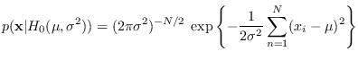
Example 4   We now expand upon the previous example by using a floating reference hypothesis and a CLT approximation for the denominator PDF. The feature $z_0$ was Gaussian, with mean $\mu$ and variance $\sigma^2/N$. Therefore the PDF obtained using the CLT is the same as the true PDF. But, for $z_1$, we need to compute the mean and variance under $H_0(\mu, \sigma^2)$. In particular, the expected value of $z_1$ is $\sigma^2$ and the variance is $2\sigma^4/(N-1)$ (See Section 17.1.2). The theoretical Chi-square PDF and Gaussian PDF based on the CLT are plotted together for $N=100$ in Figure 2.3. There is close agreement near the central peak. And while not visible in the PDF plot (top panel), there are huge errors in the tail regions visible on the log-PDF plot (bottom panel). Using the CLT PDF estimate in place of the Chi-square distribution, we obtain a J-function estimate. Figure 2.4 shows the result of comparing the J-function using a CLT PDF estimate with the exact J-function. We used Gaussian data with variance and mean chosen at random (not corresponding to $H_0$). We used a floating reference hypothesis ( $\mu=z_0, \; \sigma^2=z_1)$. The error is on the order 1e-3 for log-J function values ranging from -400 to 200! It is clear that using the floating reference hypothesis makes the approach feasible. See software/test_chisq_clt.m.

Figure 2.3: Example of Gaussian CLT approximation (red dotted) with true Chi-square PDF (blue solid).

Figure: Example of J-function estimation using CLT approximation. Horizontal axis is the true log-J function and the vertical axis is the CLT approximation. Clearly the CLT approximation is very bad when used with a fixed $H_0$ but very good when used with a floating reference hypothesis.

Since we position $H_0$ near or at the maximum of $p({\bf x}\vert H_0)$, we may ask whether there is a relationship to maximum likelihood (ML). We will explore the relationship of this method to asymptotic ML theory in a later section. To indicate the dependence of $H_0$ on ${\bf z}$, we adopt the notation $H_0$$({\bf z})$. Thus,

$$G({\bf x}; H_0 \mbox{\small$({\bf z})$} , T,g) = {p_x({\bf x}\vert H_0\mbox{\small$({\bf z})$}) \over p_z... ...all$({\bf z})$})} g({\bf z}) \;\;\;\; \mbox{ where } \;\;\; {\bf z}=T({\bf x}).$$ (2.15)

The existence of ${\bf z}$ on the right side of the conditioning operator $\vert$ is admittedly a very bad use of notation, but is done for simplicity.

In many problems, the ROS ${\cal H}_z$ is not easily found and we must be satisfied with an approximate ROS. In this case, there is a weak dependence of $J({\bf x};H_0,T)$ upon $H_0$. This dependence is generally unpredictable unless, as we have suggested, $H_0$$({\bf z})$ is always chosen to maximize the numerator PDF. Then, the behavior of $J({\bf x};H_0,T)$ is somewhat predictable. By maximizing the numerator, the result is often a positive bias. This positive bias is most notable when there is a good match to the data - a desirable feature.

Another example of the use of the CLT is provided in section 5.2.4.