Energy Statistic (ES)
In the second case above, when  is not constrained to a compact set,
and we are not willing to assume a fixed scale parameter,
the condition (3.4) must be satisfied.
To do this, we need to insure that
is not constrained to a compact set,
and we are not willing to assume a fixed scale parameter,
the condition (3.4) must be satisfied.
To do this, we need to insure that
 contains an energy statistic [3].
An energy statistic is a statistic, usually scalar, that
contains information about the norm (size) of .
The energy statistic can be explicitly included as a
component of
contains an energy statistic [3].
An energy statistic is a statistic, usually scalar, that
contains information about the norm (size) of .
The energy statistic can be explicitly included as a
component of  , such as a sample variance,
but does not need to be known explicitly.
The important thing is that if
, such as a sample variance,
but does not need to be known explicitly.
The important thing is that if
 contains an energy
statistic, then (3.4) is satisfied
for some norm. A norm
contains an energy
statistic, then (3.4) is satisfied
for some norm. A norm
 must meet the properties of
scalability (
must meet the properties of
scalability (
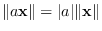 ),
triangle inequality (
),
triangle inequality (
 ),
and zero property
),
and zero property
 .
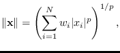
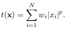
Examples of norms are generalized sample moments
.
Examples of norms are generalized sample moments
where  and
and  .
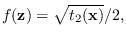
The corresponding ES is, for example
.
The corresponding ES is, for example
 |
(3.6) |
By insuring that contains an energy statistic,
then for any fixed finite-valued feature value ,
is fixed, therefore the manifold
 , in
(2.4), is compact.
This is necessary to insure the MaxEnt property [3].
Also necessary for the maxEnt property is satisfying (3.5)
for some function
, in
(2.4), is compact.
This is necessary to insure the MaxEnt property [3].
Also necessary for the maxEnt property is satisfying (3.5)
for some function  , which means that
 depends
on only through
.
Given that
depends
on only through
.
Given that
 exists,
then it is easy to find a reference hypotheses
exists,
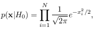
then it is easy to find a reference hypotheses  that meets
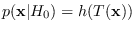
(3.5). One example can be written
that meets
(3.5). One example can be written
![$\displaystyle p({\bf x}\vert H_0) = \frac{1}{C} e^{-[f(T({\bf x}))]^p},$](img343.png) |
(3.7) |
for , and  is the apropriate scale factor.
Example 7
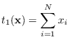
The statistic
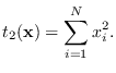 |
(3.10) |
leads to the 2-norm on
 and can be paired with the Gaussian
 |
(3.11) |
where
 and
and  .
.
Further examples of energy statistics and associated canonical
reference hypotheses are provided in Table 3.1.
Interestingly, no matter which reference hypothesis meets
(3.5) the resulting projected PDF is the same.
So, if
 ,
and
,
and
 ,
then
,
then
We will explain this in Section 3.2.3.
Table:
Reference PDFs and their energy statistics.
The reference PDFs depend on the data only through the
indicated energy statistics. Note that
 is the positive
quadrant of
where all elements of are positive
and
is the positive
quadrant of
where all elements of are positive
and
 is the hypercube
where all elements of are in
is the hypercube
where all elements of are in ![$[0,1]$](img9.png) .
.
| Name |
Data range |
Ref. Hyp.
|
Energy Statistic |
| Gaussian |
 |
 |
 |
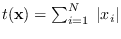
| Laplacian |
|
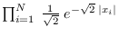 |
 |
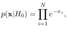
| Exponential |
 |
 |
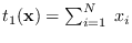 |
 |
|
 |
![$\left[\begin{array}{l}
\sum_{i=1}^N \; \log x_i \\
\sum_{i=1}^N \; x_i
\end{array}\right]$](img366.png) |
| Uniform |
 |
 |
n/a |
|