Generation of Samples from

Indeed,
is a generative model.
In this book, we will continually discuss
the generative process of creating synthetic samples of
 by drawing samples from
.
Generation of data from
is accomplished
using the following process ([3], Section 2.1)
by drawing samples from
.
Generation of data from
is accomplished
using the following process ([3], Section 2.1)
- Draw a sample
 from
from
 ,
,
- Determine the manifold
 ,
which is the set of all points
that map to through transformation
,
which is the set of all points
that map to through transformation
 :
:
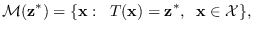 |
(2.4) |
where  is the set of valid input data samples
.
It is common to call
a manifold or level set
2.2.
is the set of valid input data samples
.
It is common to call
a manifold or level set
2.2.
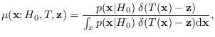
- draw a sample from
according to a distribution
proportional to
 .
.
Note that drawing a sample from
according to a distribution
proportional to
can be regarded as a a posteriori
distribution of given  . But, it is not a proper
distribution since all its probability mass exists on
which has zero volume, and so must have infinite value.
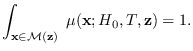
If we restrict our analysis just to the set
, we can
write down a representative distribution, called
the manifold distribution
. But, it is not a proper
distribution since all its probability mass exists on
which has zero volume, and so must have infinite value.
If we restrict our analysis just to the set
, we can
write down a representative distribution, called
the manifold distribution
 ,
,
 |
(2.5) |
where
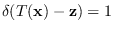 when
when
 and is zero
otherwise. Clearly
and is zero
otherwise. Clearly
Intuitively, the manifold distribution is just a distribution
on
that is proportional to
.
Subsections