Next: Energy Statistic (ES) Up: Mathematical description of MaxEnt Previous: Mathematical description of MaxEnt Contents
When ![]() is itself a compact set,
such as the unit hypercube
is itself a compact set,
such as the unit hypercube
![]() for
for
![]() ,
we can make
,
we can make
![]() the uniform
distribution. Then, so long as the manifold
the uniform
distribution. Then, so long as the manifold
![]() is compact for all
is compact for all ![]() 3.1,
then
3.1,
then
![]() will be a proper uniform distribution
for all
will be a proper uniform distribution
for all ![]() , which has maximum entropy.
Alternatively, when
, which has maximum entropy.
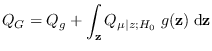
Alternatively, when ![]() is infinite in extent,
the manifold can be forced to be compact by the inclusion of an
energy statistic in
is infinite in extent,
the manifold can be forced to be compact by the inclusion of an
energy statistic in ![]() (first proposed in [3]).
The solution for compact
(first proposed in [3]).
The solution for compact ![]() and the solution for unbounded
and the solution for unbounded ![]() are formalized by the following two theorems.
are formalized by the following two theorems.
The second case considers when ![]() is not compact.
The central problem in choosing the maximum entropy reference hypothesis
when
is not compact.
The central problem in choosing the maximum entropy reference hypothesis
when ![]() is not compact
is that entropy of a distribution can go to infinity unless something is done
to constrain it. There are two approaches:
is not compact
is that entropy of a distribution can go to infinity unless something is done
to constrain it. There are two approaches:
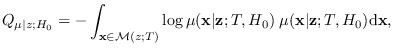
The highest-entropy distribution, which is found by maximizing the entropy of
![]() over
over ![]() , is denoted by
, is denoted by
![]() .
Intuitively,
.
Intuitively,
![]() has the
MaxEnt property because all samples generated by
has the
MaxEnt property because all samples generated by
![]() for a given
for a given ![]() are equally likely
(the uniform distribution,
which has maximum entropy on a compact set).
This is a result of the fact that
for a given
are equally likely
(the uniform distribution,
which has maximum entropy on a compact set).
This is a result of the fact that
for a given ![]() , all samples
, all samples ![]() on the manifold
on the manifold
![]() have constant value on
have constant value on
![]() ,
making
,
making
![]() also constant on the manifold,
implying that the manifold distribution is in fact the uniform distribution.
The reader is referred to a previous article for additional
details of the proof [3].
also constant on the manifold,
implying that the manifold distribution is in fact the uniform distribution.
The reader is referred to a previous article for additional
details of the proof [3].