General solution using CLT (module_A_chisq_clt.m)

The SPA is the preferred solution to solve for $p({\bf z}\vert H_0)$, but for completeness, and to serve as a comparison of the SPA approach, we cover the CLT solution. Because we intend to use the CLT to approximate $p({\bf z}\vert H_0)$, we need to use a floating reference hypothesis, (See Sections 2.3.3 and 2.3.4) $H_0({\bf z})$ and corresponding J-function

$$J({\bf x}) = \frac{p({\bf x}\vert H_0\mbox{\small$({\bf z})$})} {p({\bf z}\vert H_0\mbox{\small$({\bf z})$})}.$$

We seek a $H_0$$({\bf z})$ such that the mean of ${\bf z}$ under $H_0$$({\bf z})$ is equal to or close to the given feature value, which we designate ${\bf z}^*$. There are two possible methods. For arbitrary matrices ${\bf A}$, this can be done by projecting the input vector upon the column space of ${\bf A}$,

$$\bar{{\bf x}}={\bf A} ({\bf A}^\prime{\bf A})^{-1} {\bf A}^\prime {\bf x},$$

or

$$\bar{{\bf x}}={\bf A} ({\bf A}^\prime{\bf A})^{-1} {\bf z}^*.$$

This will satisfy the constraint ${\bf A}^\prime \bar{{\bf x}}={\bf z}^*$, however may be invalid if it has negative values.

The problem of negative values can be solved by finding a suitable positive-valued approximation, using quadratic programming to find the positive-valued (non-zero) $\bar{{\bf x}}$ that minimizes $\bar{{\bf x}}^\prime \bar{{\bf x}}$ under the constraint that ${\bf A}^\prime \bar{{\bf x}}={\bf z}^*$. For example MATLAB optimization toolkit has quadprog.m which solves the above problem with the syntax

   x = quadprog(eye(N),zeros(N,1),[],[],A',z,meps*ones(N,1));

where meps is a small positive number (minimum allowed value of $\bar{x}_i$). A good $\bar{{\bf x}}$ also results if we minimize the spectral entropy

$$Q_s({\bf x}) = \sum \log \bar{x}_i$$ (5.5)

under the same constraints.

Another particularly elegant solution to find $\bar{{\bf x}}$ can be found in time-series analysis where we use the autoregressive spectrum estimate for $\bar{{\bf x}}$. We will discuss this in section 5.2.5.

Regardless of which method we used to obtain $\bar{{\bf x}}$, let $H_0$$({\bf z})$ be the hypothesis that ${\bf x}$ has mean $\bar{{\bf x}}$, with $\bar{{\bf x}}$ satisfying (or nearly satisfying) the constraint ${\bf A}^\prime \bar{{\bf x}}={\bf z}^*$. Therefore, under $H_0$$({\bf z})$, the mean of ${\bf z}$ is near to ${\bf z}^*$ itself. In section 2.3.3, we discussed the concept of the region of sufficiency (ROS).

When applying the central limit theorem, we need only consider the mean and variance of $x_i$. For the chi-squared RV, the mean is $\bar{x}_i$ and the variance is $q_i = \left(\frac{2}{k_i}\right) (\bar{x}_i)^2$. The mean of ${\bf z}$ is therefore

$$\bar{{\bf z}}={\bf A}^\prime \bar{{\bf x}}.$$

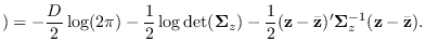
The covariance of ${\bf z}$ under $H_0$$({\bf z})$ is

$${\bf\Sigma}_z = {\bf A}^\prime \; \Lambda_z \; {\bf A},$$

where $\Lambda_z$ is the diagonal matrix with diagonal elements $q_i$. We can immediately write down the J-function denominator,

$$\log p({\bf z}\vert H_0$$$({\bf z})$$$) = -\frac{D}{2} \log(2\pi) -{1\over 2}\log {\rm det}( {\bf\Sigm... ...1}{2}({\bf z}-\bar{{\bf z}})^\prime {\bf\Sigma}_z^{-1} ({\bf z}-\bar{{\bf z}}).$$

If $\bar{{\bf z}}={\bf z}$, then the last term disappears.

Example 9   We now re-examine example 8, however this time we apply the CLT method. Once again, projected PDF values are plotted against the true values of $p({\bf x}\vert H_a)$ in Figure 5.3. The acid test passes. The function software/module_A_chisq implements reature trasformation and J-function. The function software/module_A_chisq_test.m runs the acid test (with variable CLT set to 1) using syntax:

       module_A_chisq_test('acid',100,2,2,”,1);

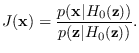
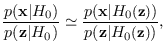
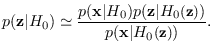
It is interesting to compare the Jout values from the SPA and CLT methods. In Figure 5.4, we see there is close agreement. Mathematically, we have

$${p({\bf x}\vert H_0) \over p({\bf z}\vert H_0)} \simeq {p({\bf ... ...0\mbox{\small$({\bf z})$}) \over p({\bf z}\vert H_0\mbox{\small$({\bf z})$})},$$

where the right hand side is the J-function from the CLT method using the floating reference hypothesis. Clearly then,

$$p({\bf z}\vert H_0) \simeq { p({\bf x}\vert H_0) p({\bf z}\vert ... ...mbox{\small$({\bf z})$}) \over p({\bf x}\vert H_0\mbox{\small$({\bf z})$}) } .$$

Note that this provides an alternative to the SPA for computing the PDF of ${\bf z}$ under a fixed reference hypothesis.

Figure 5.3: Acid test results for module_A_chisq_clt.m.

Figure 5.4: Jout comparison for SPA and CLT.