Next: Application of CLT to Up: J-function Implementations Previous: General solution using CLT Contents
The main problem in CLT is finding a positive-valued
mean for the floating reference hypothesis,
![]() ,
for which the feature mean is equal to the current
feature value. Let
,
for which the feature mean is equal to the current
feature value. Let ![]() be the current ACF feature value.
We need to find a positive-valued
be the current ACF feature value.
We need to find a positive-valued
![]() such that
such that
![]() A convenient approach comes from AR analysis,
where it is known that the ACF of the
AR spectrum is equal to the original ACF [31].
Thus, the AR spectral estimate serves as
A convenient approach comes from AR analysis,
where it is known that the ACF of the
AR spectrum is equal to the original ACF [31].
Thus, the AR spectral estimate serves as
![]() .
.
Using the Levinson-Durbin recursion [31], we may transform
the ACF ![]() into the AR coefficients
into the AR coefficients
![]() ,
and
,
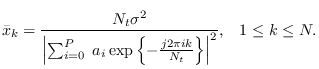
and ![]() . The corresponding AR spectrum is written
. The corresponding AR spectrum is written
Under
![]() , the elements of
, the elements of ![]() are independent and Chi-squared with 1 or 2 degrees of freedom with mean
are independent and Chi-squared with 1 or 2 degrees of freedom with mean
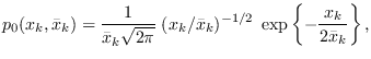
![]() (See Section 17.1.2). Bins
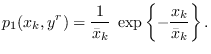
(See Section 17.1.2). Bins ![]() are distributed according to
are distributed according to
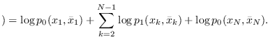
In summary, we take the following steps:
     % Nt = FFT size
     % x is dimension n by 1, where n=Nt/2+1;
     % A is dimension n by P+1
     % k is vector of degrees-of-freedom
     k = [1;2*ones(n-2,1); 1];
     A = cos([0:Nt/2]' *(2*pi/Nt)*[0:P]).*repmat(k,1,P+1)*(1/Nt^2);
z=A'*x;
[a,e]=levinson(z);
The output variable e is the AR innovation variance parameter
  af = fft(a(:),Nt);
  xz = Nt * e  ./ abs(af(1:n)).^2;
lpxHz = expon_dist(x([2:n-1],:),xr([2:n-1],:)) + ...
    chisq1_dist(x([1 n],:),xr([1 n],:));
   format long
   [A'*xr z]
q = 2./k .* xz.^2;The covariance of
Sz = A'*diag(q)*A;Then,
    ldetSr=log(det(Sz));
    lpzHz =  -(P+1)/2*log(2*pi) - .5*ldetSz;
See
software/module_acf_clt.m for additional details.
Use
software/module_acf_synth.m for inversion (re-synthesis).
The module can be tested using
software/module_acf_test.m with TYPE=1.
We compare this method with other approaches in Section 10.4.10.