Application of SPA to Circular Auto-Correlation Function Analysis

The auto-correlation function (ACF) is widely used in auto-regressive (AR) time-series analysis and spectral estimation [31]. An estimate of the ACF given a length-$N_t$ time-series can be obtained using the frequency-domain approach by inverse DFT of the raw spectrum. Because the FFT is used, this approach falls under feature extraction methods for circularly stationary processes (See section 10.1). The “input" data ${\bf x}$ is the $N\times 1$ vector of raw spectral values (magnitude-squared DFT), where $N=N_t/2+1.$ The output ACF feature is ${\bf z}={\bf A}^\prime {\bf x}$. To compute the $P$-th order ACF (lags 0 through $P$), the columns of the $N\times(P+1)$ matrix ${\bf A}$ must contain the cosine functions which are the basis functions for the real part of the inverse FFT. To properly compute the ACF, we need to effectively compute the inverse-FFT of the full length-$N_t$ spectrum (redundant bins duplicated) which requires that we scale the complex bins ( $i=\{2,3 \ldots N-1\}$) by 2.0 and the real bins ($i=\{1,N\}$) by 1.0. This un-equal bin scaling can be formalized by the scaling variable $w_i$, which takes the values of 1 or 2 as indicated. The resulting transformation is

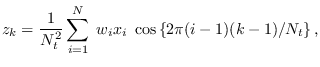$$z_k = \frac{1}{N_t^2} \sum_{i=1}^{N} \; w_i x_i \; \cos\left\{ 2 \pi (i-1) (k-1)/N_t\right\},$$ (5.4)

for $1\leq k \leq P+1.$ This computes the order-$P$ circular ACF using the frequency-domain method. In this case, the energy statistic is $t({\bf x}) = \sum_i \; w_i x_i,$ with un-equal bin scaling, which is a valid norm on ${\cal P}^N$.

There are two possibilities for computation of the ACF depending on if one is starting with time-series or spectral data. In both cases, we may assume that the time-series is independent Gaussian noise with mean 0 and variance 1. If ${\bf x}$ is the time-series, then $p({\bf x}\vert H_0)$ is taken directly from Table 3.1, “Gaussian" row, and $p({\bf z}\vert H_0)$ is computed using software/pdf_A_chisq_m.m.

   [lpzH0,ic] = pdf_A_chisq_m(z,A,K,[ic]);

where K is an $N\times 1$ vector with the degrees of freedom [1,2,2, ... 2,2,1]. See software/module_acf_spax.m for additional details. For testing, use software/module_acf_test.m with TYPE=2.

If ${\bf x}$ is the raw spectrum, $p({\bf x}\vert H_0)$ is given by (4.1), with ${\bf x}$ taking the role of ${\bf z}$ in the equation, and $p({\bf z}\vert H_0)$ is computed using software/pdf_A_chisq_m.m. For additional details, see software/module_acf_spa.m. For re-synthesis, use software/module_acf_synth.m. For testing, use software/module_acf_test.m with TYPE=0.