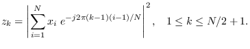
Magnitude Squared DFT of Gaussian data
This building block considers the DFT of Gaussian data followed by the
computation of the magnitude-squared of the bins.
Like the previous example, this belongs to a general class of chi-squared
feature extractors fitting within the “Gaussian" row of Table 3.1.
The energy statistic in all of these problems is the total energy.
In the case of DFT magnitude-squared,
the ES is contained implicitly (Parseval's theorem).
Let  be even and
The DFT bins are independent under  , but not identically
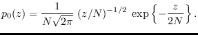
distributed. DFT bins 0 and
, but not identically
distributed. DFT bins 0 and  are real-valued so
 have the Chi-squared distribution with 1 degree of freedom
scaled by , which we denote by
have the Chi-squared distribution with 1 degree of freedom
scaled by , which we denote by  :
:
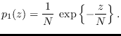
DFT bins 1 through  are complex
so have the Chi-squared
distribution with 2 degrees of freedom scaled by ,
which we denote by
are complex
so have the Chi-squared
distribution with 2 degrees of freedom scaled by ,
which we denote by  :
:
The complete PDF
 is
is
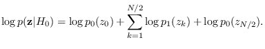 |
(4.1) |
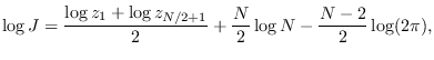
The J-function,
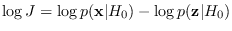 can be simplified for even to
which interestingly is data independent except with respect to the zero
and Nyquist frequency bins.
For more information, refer to the software module
software/module_dftmsq.m.
Re-synthesis of  from
from  using UMS (Section 3.3)
is accomplished first by taking the square-root
of each bin. We then multiply the zero and Nyquist
bins (
using UMS (Section 3.3)
is accomplished first by taking the square-root
of each bin. We then multiply the zero and Nyquist
bins ( and
and  for even ) by 1 or -1,
each with probability 1/2.
The remaining bins are multiplied by a phase term
for even ) by 1 or -1,
each with probability 1/2.
The remaining bins are multiplied by a phase term
 , where
  are independent RV uniformly
distributed on the interval
are independent RV uniformly
distributed on the interval
![$[0,\;2\pi]$](img414.png) .
Finally, the length- DFT vector is created
by appending the conjugate of the complex bins, then
taking the inverse DFT to obtain .
For more information, refer to the software module
software/module_dftmsq_synth.m.
.
Finally, the length- DFT vector is created
by appending the conjugate of the complex bins, then
taking the inverse DFT to obtain .
For more information, refer to the software module
software/module_dftmsq_synth.m.