Consider the transformation
Although dimension-preserving, the sign of the input
data is lost. This problem clearly belongs to the “Gaussian"
row in Table 3.1 since the
associated energy statistic can indeed be
computed from  . The PDF
 is found
in the “Gaussian" row in Table 3.1,
from which we have
is found
in the “Gaussian" row in Table 3.1,
from which we have
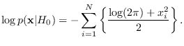
Under  , is a set of independent
Chi-square RV with one degree of freedom
(See Section 17.1.2), therefore,
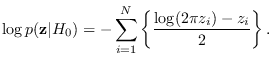
, is a set of independent
Chi-square RV with one degree of freedom
(See Section 17.1.2), therefore,
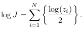
Performing the calcellations in
we get
For more information, refer to the software module
software/module_square.m.
Re-synthesis of  using UMS (Section 3.3) from
is accomplished by assigning
using UMS (Section 3.3) from
is accomplished by assigning
where sign  takes a value of
  or
or  , each with probability 1/2.
For more information, refer to the software module
software/module_square_synth.m.
, each with probability 1/2.
For more information, refer to the software module
software/module_square_synth.m.