The Fixed Reference Hypothesis and the PDF tail problem

Under normal sitiations, it is highly unlikely, that the data ${\bf x}$ lies near the central peak of $p({\bf x}\vert H_0)$. It is far likelier that it is in the far tails. This will cause the numerator and denominator PDFs in (2.3) to approach zero. Representing the PDF value may be well below the machine precision. But, as long as the log of $p({\bf x}\vert H_0)$ and $p({\bf z}\vert H_0)$ may be represented accurately, this is not an issue, as all calculations of this sort can (and should) be done in the log domain. As the reader will discover through experience, as ${\bf x}$ varies over a wide range of values, there may be large variations in the individual terms, but by and large, the difference $\log p({\bf x}\vert H_0) - \log p({\bf z}\vert H_0)$ remains within fairly reasonable range of values.

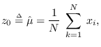
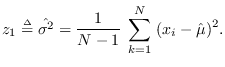
Example 1   We now consider the feature set pair consisting of the sample mean and variance ${\bf z}= [z_0, z_1]$, where

$$z_0 \stackrel{\mbox{\tiny$\Delta$}}{=}\hat{\mu} = \frac{1}{N} \; \sum_{k=1}^N \; x_i,$$

$$z_1 \stackrel{\mbox{\tiny$\Delta$}}{=}\hat{\sigma^2} = \frac{1}{N-1} \; \sum_{k=1}^N \; (x_i-\hat{\mu})^2.$$

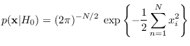
Let $H_0$ be the hypothesis that ${\bf x}$ is a set of $N$ independent identically distributed Gaussian samples with mean 0 and variance 1. We have

$$p({\bf x}\vert H_0) = (2\pi)^{-N/2} \; \exp\left\{ -\frac{1}{2} \sum_{n=1}^N x_i^2 \right\}$$ (2.11)

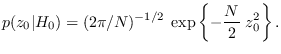
It is well known [15] that under Gaussian $H_0$ $\hat{\mu}$ and $\hat{\sigma^2}$ are statistically independent, so they can be treated separately. Furthermore, under $H_0$, $z_0$ is Gaussian with mean 0 and variance $1/N$, thus

$$p(z_0 \vert H_0) = (2\pi/N)^{-1/2} \; \exp\left\{ -\frac{N}{2} \; z_0^2 \right\}.$$

Also, $\hat{\sigma}^2$ is a chi-square RV with $N-1$ degrees of freedom derived from a zero-mean Normal distribution with variance $\frac{1}{N-1}$ (See Section 17.1.2), thus

$$p(z_1 \vert H_0) = (N-1) \; \Gamma^{-1}\left({N-1\over 2}\right) ... ...{z_1 (N-1)} \right)^{(N-1)/2-1} \; \exp\left\{ -{z_1 (N-1) \over 2 } \right\}$$

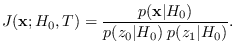
Finally, for the J-function we have

$$J({\bf x}; H_0,T) = {p({\bf x}\vert H_0)\over p(z_0 \vert H_0) \; p(z_1 \vert H_0)}.$$

We simulated this example using $N=128$ . Data was created with mean uniformly distributed between -5 and 5, and variance uniformly distributed from 0 to 100. In ten random trials, $p({\bf x}\vert H_0)$ and $p({\bf z}\vert H_0)$ numerically underflowed (evaluated to zero) nine of the ten times. When the log-PDFs were evaluated instead, the log-PDF values ranged across a wide range from -7000 to -629. The log-J function ranged from -448 to -310. See software/test_mv.m.

In the above example, an analytic expression is available for $\log p({\bf z}\vert H_0)$. This is not the case in general. The types of transformations and reference hypotheses for which analytic expressions are available are limited. We will see in the following sections how these problems can be alleviated.