The Saddle Point Approximation
As we stated in the last section, the types of transformations and reference hypotheses
for which analytic expressions are available are limited.
For a broader class of statistics,
the exact moment generating function (MGF) is often known.
The problem is that inversion of the MGF transformation to find the exact PDF
may not be possible in closed form. For these cases, we
can use the saddle point approximation (SPA) which provides accurate
tail PDF estimates. Steven Kay was the first to recommend the
saddle point Approximation as a solution to this problem in CSM.
Later, it was futher developed by Nuttall [16].
It should be kept in mind that although the SPA
is an approximation, approximation errors can be ignored for all
practical purposes [1].
Furthermore, the accuracy is not degraded in the PDF tails.
On the contrary, it is extremely well adapted to the task at hand, even for
input data very far from the central peak of the reference hypothesis PDF.
This is because the SPA approximates the
shape of the integrand, not the value (height) of it.
There are limits, however
and we find that the SPA, which is a recursive search for the
saddle point itself, may suffer from convergence problems.
This problem is solved using the data normalization, which is a special case
of a floating reference hypothesis and is described in section 2.3.4.
Further details about the SPA are provided in Appendix 17.6.
Let feature
 .
The moment-generating function for
.
The moment-generating function for
 is given by
for  -dimensional Laplace transform variable
 .
Then,
.
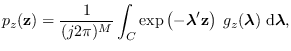
Then,  is obtained by the inverse Laplace transform:
where
 The contour
  is parallel to the imaginary axis in each of the
  dimensions of
.
The joint cumulant generating function (CGF) is
dimensions of
.
The joint cumulant generating function (CGF) is
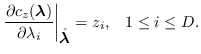
For a specified , the saddle point is that real point
 where all partial derivatives satisfy
The saddle point may be found iteratively using the recursion
where

 is the gradient vector of
 w/r to
, and
w/r to
, and
 is the
  matrix
of second partial derivatives
matrix
of second partial derivatives
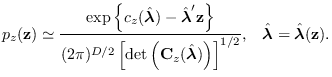
Once the saddle point
is found,
the saddle point approximation is given by
 |
(2.12) |
Example 2
Let  be a set of
  samples of positive-valued
data, such as intensity or power spectrum measurements.
Let
samples of positive-valued
data, such as intensity or power spectrum measurements.
Let
 , where
matrix
, where
matrix  is
is  .
This is a simple linear operation producing the
-dimensional feature .
To compute the J-function for this
feature transformation, we need to select
a reference hypothesis
.
This is a simple linear operation producing the
-dimensional feature .
To compute the J-function for this
feature transformation, we need to select
a reference hypothesis
 for which we can compute
the feature PDF
for which we can compute
the feature PDF
 .
We are tempted to use the Gaussian PDF
since the Gaussian PDF of would be trivial to derive.
Although (2.2) would result in a valid projected PDF,
.
We are tempted to use the Gaussian PDF
since the Gaussian PDF of would be trivial to derive.
Although (2.2) would result in a valid projected PDF,
 would have support for negative
values of , which would violate our prior knowledge
that was positive. Other reasons why this is a bad choice
of
would have support for negative
values of , which would violate our prior knowledge
that was positive. Other reasons why this is a bad choice
of  are discussed on chapter 3.
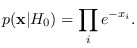
A much better choice is the exponential PDF
(1/2 times the standard
are discussed on chapter 3.
A much better choice is the exponential PDF
(1/2 times the standard  random variable
: chi-square distribution with 2 degrees of freedom, scaled by 0.5)
random variable
: chi-square distribution with 2 degrees of freedom, scaled by 0.5)
Unfortunately, the PDF
is not known in closed
form. This problem was adressed in
2000 by Steven Kay who suggested the use of the saddle point approximation
(SPA) [16].
Although
is not known in closed
form, the moment generating function (MGF) is known.
Is is just a matter of numerical inversion of the MGF.
We address this problem in detail in Section 17.6.
The function software/pdf_A_chisq_m.m implements
the algorithm that computes
 .
.
To test the approach, we generated data
as independent samples of from the distribution,
for  , then used the matrix
We compared the histogram of the values of with the
SPA for each histogram bin. Figure 2.2 shows the result.
Figure 2.2:
Comparing histogram with PDF approximated using SPA.
|
|
The saddle point approximation is used in many examples in this book.
These examples include
sections 17.6, 17.7.1, 9.1.2, 2.3.2,
and 5.2.1.
![$\displaystyle {\bf C}_z(\lambda) \stackrel{\mbox{\tiny $\Delta$}}{=}\left[ \frac{\partial^2c_z(\lambda)}{\partial \lambda_l \partial \lambda_m}\right].$](img172.png)
![$\displaystyle {\bf A}=\left[ \begin{array}{ll} 1 & 0\\
1 & 1\\
1 & 2\\
1 & 3\\
\vdots & \vdots \\
1 & N-1
\end{array}\right]
$](img178.png)
![\includegraphics[height=3.5in,width=6.0in]{test_spa.eps}](img179.png)