Saddlepoint Approximation
Since no closed-form expression for the joint PDF of  in (9.1) is known,
we apply the Saddlepoint approximation
[55],[16].
To obtain the SPA, we need the joint cumulant
generating function (CGF) of , namely,
in (9.1) is known,
we apply the Saddlepoint approximation
[55],[16].
To obtain the SPA, we need the joint cumulant
generating function (CGF) of , namely,
where


 is the
joint moment-generating function (MGF) of .
Also, we need the first and second-order partial derivatives
of
is the
joint moment-generating function (MGF) of .
Also, we need the first and second-order partial derivatives
of
 .
Once these are known, the formulas in reference [16]
may be used to obtain the SPA.
.
Once these are known, the formulas in reference [16]
may be used to obtain the SPA.
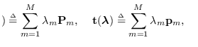
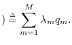
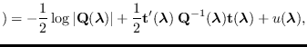
It is shown in [56] that
where
with
and
The first-order partial derivatives are
for
 ,
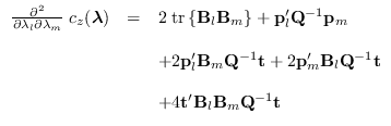
and the second-order partial derivatives are
,
and the second-order partial derivatives are
where
and we drop the
 dependence
from
dependence
from
 ,
,
 ,
and
,
and
 , for simplicity.
The third and fourth derivatives, necessary
for the first-order correction term of the
SPA have also been worked out
[56].
, for simplicity.
The third and fourth derivatives, necessary
for the first-order correction term of the
SPA have also been worked out
[56].
The equations simplify considerably if we assume
that
 and
and  are all zero
and compute the PDF under the WGN assumption
are all zero
and compute the PDF under the WGN assumption  .
We then have
.
We then have
The first order partial derivatives reduce to
and the second order partial derivatives become
The SPA algorithm is provided in
software/pdf_quadspa.m,
which assumes that
and are all zero
and computed the PDF under the WGN () assumption.