Maximum likelihood and PDF Projection
We have stated that when we use a floating reference hypothesis,
we prefer to choose the reference hypothesis such that the numerator of the J-function
is a maximum. Since we often have parametric forms for the PDFs, this amounts to finding
the ML estimates of the parameters.
If there are a small number of features,
all of the features are ML estimators for
parameters of the PDF, and there is sufficient data to guarantee
that the ML estimators fall in the
asymptotic (large data) region, then
the floating hypothesis approach
is equivalent to an existing approach
based on classical asymptotic ML theory.
We will derive the well-known asymptotic result
using (2.15).
Two well-known results from asymptotic theory
[17] are the following.
- Subject to certain
regularity conditions (large amount of data,
a PDF that depends on a finite number of parameters
and is differentiable, etc.), the PDF


 may be approximated by
where
 is an arbitrary value of the parameter,
 is the maximum likelihood estimate
(MLE) of
, and
is the maximum likelihood estimate
(MLE) of
, and

 is the Fisher's information
matrix (FIM) [17].
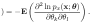
The components of the FIM for PDF parameters
is the Fisher's information
matrix (FIM) [17].
The components of the FIM for PDF parameters
 are given by
The approximation is valid only for
in the vicinity
of the MLE (and the true value).
- The MLE
is approximately
Gaussian with mean equal to the true value
and covariance equal to
 , or
, or
 |
(2.19) |
where  is the dimension of
.
Note we use
in evaluating the FIM in place of
,
which is unknown. This is allowed because
has a weak dependence on
.
The approximation is valid only for
in the vicinity
of the MLE.
is the dimension of
.
Note we use
in evaluating the FIM in place of
,
which is unknown. This is allowed because
has a weak dependence on
.
The approximation is valid only for
in the vicinity
of the MLE.
To apply equation (2.15),
takes the place of  and
and

 is the hypothesis that
is the true
value of
. We substitute (2.18)
for
is the hypothesis that
is the true
value of
. We substitute (2.18)
for
 and (2.19) for
 .
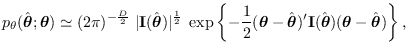
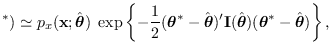
Under the stated conditions,
the exponential terms in approximations (2.18),(2.19)
become 1. Using these approximations, we arrive at
.
Under the stated conditions,
the exponential terms in approximations (2.18),(2.19)
become 1. Using these approximations, we arrive at
![$\displaystyle \hat{p}_x({\bf x}\vert H_1) = \left[{ p_x({\bf x}; \hat{\mbox{\bo...
...ac{1}{2}} }
\right] \; \hat{p}_\theta(\hat{\mbox{\boldmath$\theta$}}\vert H_1),$](img234.png) |
(2.20) |
which agrees with the PDF approximation
from asymptotic theory [18],
[19]. Equation (2.20) is very useful for integrating ML estimators
into class-specific classifier and we will give examples of its use.
The first term (in brackets) is the J-function.
To compare equations (2.15) and (2.20),
we note that for both, there is an implied sufficiency
requirement for and
, respectively.
Specifically,
must remain in the ROS of ,
while
must be asymptotically sufficient for
.
However, (2.15) is more general
since (2.20) is valid only when
all of the features are ML estimators and
only holds asymptotically
for large data records with the implication that
tends to Gaussian, while (2.15) has no such
implication. This is particularly important in
upstream processing where there has not been significant data reduction
and asymptotic results don't apply.
Using (2.15), we can make simple adjustments to the
reference hypothesis to match the data better and avoid the PDF
tails (such as controlling variance)
where we are certain that we remain in the ROS of .
Example 5
We revisit example 3 and 4, this time using the ML approach.
Note that  , and
, and
 are the ML estimates
of mean and variance [15].
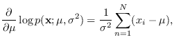
It is instructive to derive the CR bound for this problem (Section 17.5).
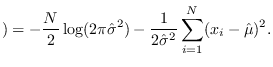
Taking the log of (2.14),
are the ML estimates
of mean and variance [15].
It is instructive to derive the CR bound for this problem (Section 17.5).
Taking the log of (2.14),
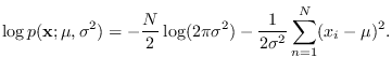 |
(2.21) |
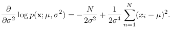
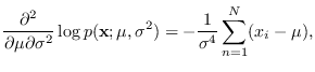
We require the first derivatives
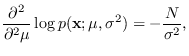
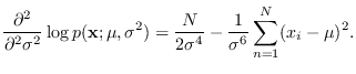
Taking second derivatives,
The next step is to take
 of the above.
Using that
of the above.
Using that
 ,
,
 ,
,
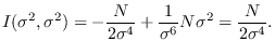
Finally, the FIM for this problem is given by
whos inverse is the CR bound
Note the close relationship to the CLT approach used in example 4.
There is essentially no difference aside from the
variance of  which is
 in the CR bound
analysis, but
in the CR bound
analysis, but
 in the CLT example.
Whenever the ML approach can be used, it is, in fact the same
as the CLT approach asymptotically as
in the CLT example.
Whenever the ML approach can be used, it is, in fact the same
as the CLT approach asymptotically as  becomes large.
We let the floating reference hypothesis
be that
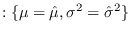 , or
in other words that the true values of
, or
in other words that the true values of  and
and  are equal
to the ML estimates. We have,
are equal
to the ML estimates. We have,
Note that
leaving
For
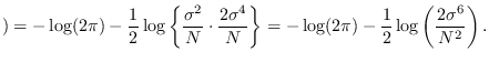
 , we have (See denominator of equation 2.20 ) that
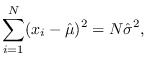
where  .
.
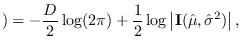
We therefore have that
We compared the J-functions using the above equations
with the J-function from the fixed reference hypothesis
(example 1). There was close agreement.
For details, see Figure 2.5 and software/test_mv_ml.m.
Figure 2.5:
Comparison of J-function from exact solution (example 1)
with ML approximation.
|
|
Another example of the use of the ML method is provided in section
5.2.8.

![$\displaystyle {\bf I}(\hat{\mu}, \hat{\sigma}^2) =
\left[ \begin{array}{cc}
\frac{N}{\sigma^2} & 0\\
0 & \frac{N}{2\sigma^4}
\end{array} \right],
$](img247.png)
![$\displaystyle {\bf C}(\hat{\mu}, \hat{\sigma}^2) =
\left[ \begin{array}{cc}
\frac{\sigma^2}{N} & 0\\
0 & \frac{2\sigma^4}{N}
\end{array} \right].
$](img248.png)
![\includegraphics[width=4.2in,height=3.9in, clip]{test_mv_ml.eps}](img262.png)