Interpretation of the J-function

The J-function is a measure of the ability of the features to describe the input data. Mathematically, the J-function is equal to the manifold density (2.5) [3]. The manifold density comes into play when we generate samples from $G({\bf x};H_0,T,g)$. For maximum entropy PDF projection (See Chapter 3), the manifold density is the uniform density (see Section 3.3). The manifold is a range of input data values that map to a given feature value. So, if the features are very descriptive, and accurately describe the peculiarities of the given data sample, the range of possible input data values shrinks, increasing the value of manifold density.

Another interpretation, based on asymptotic maximum likelihood (ML) theory, starts by assuming that there exists some parametric model $p({\bf x};$$\theta$$)$ such that the features are maximum likelihood estimates of the parameters, ${\bf z}=\hat{\mbox{\boldmath $\theta$}}$. The J-function for ML, given in (2.27), is dominated by the numerator, which is the likelihood function of the data evaluated at $\hat{\mbox{\boldmath $\theta$}}$. Thus, the J-function has the interpretation as a quantitative measure of how well the parametric model can describe the raw data. The better the features, the better this notional parametric model. Interestingly, because the J-function can be computed without actually implementing the ML estimator, this information is available without needing to know the parametric form nor needing to maximize it! Naturally, there are situations where this information is detrimental to classification - specifically if the data contains nuisance information or interference. There are work-arounds that significantly improve classification performance, for example the class-specific feature mixture ([20], section II.B).

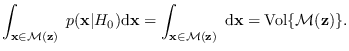
There is also a geometric interpretation that lends insight into the general approach. For the uniform reference hypothesis ( $p({\bf x}\vert H_0)=1$), (2.2) reduces to $G({\bf x}) = \frac{1}{p({\bf z}\vert H_0)}$, but $p_T({\bf z}\vert H_0)$ is just the volume of the manifold (2.4):

$$\int_{{\bf x}\in {\cal M}({\bf z})} \; p({\bf x}\vert H_0) {\rm d... ...x}\in {\cal M}({\bf z})} \; {\rm d}{\bf x}= {\rm Vol} \{ {\cal M}({\bf z}) \}.$$

Therefore, $G({\bf x})=\frac{1}{{\rm Vol} \{ {\cal M}({\bf z}) \}}$. This touches on the idea of information maximization [21]. In a general sense, maximizing information throughput of a transformation comes down to finding feature transformations with small manifolds given feature values ${\bf z}$, something that one could call back-projected volume. This interpretation is implicit in the statement by Nadal “A large amount of information is obtained if one can discriminate finely the input signal." [22]. From the point of view of unsupervised learning, when data of multiple classes is present, it makes sense that when the average back-projected volume is minimized, data becomes better separated in the output distribution. This is because a given feature value will map back to a smaller region in $\mathbb{R}^N$, which is less likely to have data of more than just one class.