One Class/One Model: Class-Specific Features (CSF)

One way to compare/combine likelihood functions is to assign a different feature extraction chain to each class assumption. This results in the CSF classifier, which is just an application of the projected PDF (2.2) as a Bayesian classifier,

$$\arg \max_k \left\{ \frac{p({\bf x}\vert H_{0,k})}{p({\bf z}\vert H_{0,k})} p({\bf z}\vert H_k) \; p(H_k)\right\}.$$ (12.4)

Notice that the reference hypotheses may be class-dependent. A reference hypothesis can be chosen for maximum entropy (Sections 3.1.1,3.2), or for suffiency (2.2.2). The implicit assumptions in (2.2) is that that feature ${\bf z}_k=T_k({\bf x})$ is a sufficient (or at least approximately sufficient) statistic for the binary test between class $H_k$ and $H_{0,k}$. Approximate sufficiency means that

$$\frac{p({\bf x}\vert H_k)}{p({\bf x}\vert H_{0,k})}\simeq \frac{p({\bf z}\vert H_k)}{p({\bf z}\vert H_{0,k})}.$$

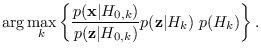
This optimality goal can be approximated individually for each class to maximize the sufficiency or minimize the dimension of the features. Take for example, sinewaves in colored noise. With a white-noise reference hypothesis, the feature set must be sufficient for “white noise" vs. “colored noise plus sinewave", so must include parameters describing the sinewaves and the background spectrum. A feature set such as the SINAR model (Section 9.2) could be used. On the other hand, if the background spectrum is known, this background spectrum (without sinewaves) would make a better choice for $H_0$. Then, the features would only need to be sufficient for “colored noise" vs. “colored noise plus sinewave", so would only need to describe the detected sinewaves.

Equation (2.2) also makes the one class, one feature assumption, where for each class, there is a “best" feature. This assumption may not be appropriate in some problems. In some cases, data is collected imprecicely, or collections of data may consist of mixtures of different physical phenomena. Or, interference or background noise may vary. In (12.4), the J-function (2.3) usually dominates, thus potentially causing classification errors for data that has characteristics better represented by a different feature. In these cases, it is better to use the class-specific feature mixture (CSFM).