Block Segmentation

Figure 12.1 shows a generalized representation of block segmentation for PDF projection-based models. The input data ${\bf x}$ is segmented in various ways. In the figure ${\bf x}$ is divided into 1, 2, 3, and 4 equal segments. In general, the segments do not need to be of uniform size. What distiguishes block segmentation from other types is the fact that the segments are non-overlapping and no window function is used (rectangular weighting). It is also important that all samples of ${\bf x}$ are included in the totality of the segments. This means that for uniform-sized segments, the input size $N$ must be an integer multiple of the segment size. For this reason, it is prudent to truncate all input data ${\bf x}$ to a multiple of some highly divisible number, such as $768$.

In Figure 12.1, each branch uses a different uniform segment size, and the same feature transformation is used for all segments in each branch. The uniform segmentation and uniform feature extraction is the most common because it lends itself to PDF estimation using HMM (Section 13.3). In general, the segmentation can be non-uniform and different feature transformations can be used within a branch. Furthermore, some branches could use the same segmentation, but different feature transformations.

Figure: Block-segmentation architecture. The same input data ${\bf x}$ is presented to each branch, where it may be differently segmented, and processed by different feature extraction transformations. The output of branch $i$ is the projected PDF $G_i({\bf x})$. The branch outputs are combined or compared.

Block segmentation is necessary for strict interpretation of the PDF projection theorem in the presence of segmented data. Let's talk about one branch in Figure 12.1. Let $K$ be the segment size, so $N=TK$, where $T$ is the number of segments. Then,

$${\bf x}=[{\bf x}_1, {\bf x}_2 \ldots {\bf x}_T].$$

Let $H_0$ be the reference hypothesis, in which the samples of ${\bf x}$ are iid, either exponential (3.9) or Gaussian (3.11). It follows that the segments are independent,

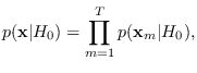$$p({\bf x}\vert H_0)=\prod_{m=1}^T p({\bf x}_m\vert H_0),$$ (12.1)

and if each segment feature is computed from the corresponding data segment, ${\bf z}_m=T({\bf x}_m)$, we have

$$p({\bf z}\vert H_0)=\prod_{m=1}^T p({\bf z}_m\vert H_0).$$ (12.2)

Then, PDF projection (2.2) is applied using (12.1) and (12.2). The joint feature PDF $g({\bf z})=g({\bf z}_1,{\bf z}_2 \ldots {\bf z}_T)$ is obtained from the HMM forward procedure (Section 13.3). Thus, block segmentation allows the exact application of PDF projection (2.2) through the strict independence of the segments under $H_0$. There are, however, significant disadvantages of block segmentation. It is not guaranteed that the segment boundaries fall at appropriate times. The occurrences of events in the data may get split into several segments, and extreme Gibbs-effect will be seen in the frequency domain. The result can be poor and erratic feature extraction. For these reasons, it may be prefereable to use overlapped/windowed segments.