AR Data PDF - exact

The exact PDF of an AR process is given by (10.6) with the ACF equal to the inverse FT of (10.40). The ACF may also be obtained (inefficiently) from the reverse Levinson algorithm

  r = rlevinson([a(:); zeros(N-P-1,1)],sig2);

In practice, we would obtain the length-$N$ ACF by the inverse DFT of the circular PSD (10.41) using a large enough transform of size $2L$ that the ACF dies to zero for $t<L$.

In the following analysis, we assume that the AR coefficients are known. The problem of computing (10.6) knowing just ${\bf R}_N$ is inherently different because we must estimate the AR coefficients (See sections 10.4.3). Efficient means of computing the exact PDF for the more general ARMA model are provided in Sections 10.2.2 and 10.2.3. The special properties of the AR model can be used to advantage. First of all, $K$, the impulse response length of the whitening filter is exactly $K=P$. Thus, only the first $P$ samples of the whitened sequence need be “corrected".

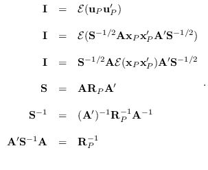
Also, a closed form expression for the inverse of the $P\times P$ ACF matrix can be found. Suppose we obtain the AR coeffients of all orders up to and including $P$. Let r(i) be the i-th ACF coefficient (lag i-1). Let Aa(p,:) be the $p-1$-th order AR coefficient vector and e(p) the corresponding prediction error variance $\sigma^2_{p-1}$ (note that $\sigma^2_P = \sigma^2$) :

  Aa = zeros(P+1,P+1);
  for p=1:P+1,
         [Aa(p,1:p),e(p)]=levinson(r(1:p));
  end;

Now consider the operation :

  u(1) = (x(1)*Aa(1,1))/sqrt(e(1));
  u(2) = (x(2)*Aa(2,1) + x(1)*Aa(2,2))/sqrt(e(2));
  :            :
  u(P) = (x(P)*Aa(P,1) + ...  + x(1)*Aa(P,P))/sqrt(e(P));
  u(P+1) = (x(P+1)*Aa(P+1,1) + ...  + x(1)*Aa(P+1,P+1))/sqrt(e(P+1));
  u(P+2) = (x(P+2)*Aa(P+1,1) + ...  + x(2)*Aa(P+1,P+1))/sqrt(e(P+1));
  u(P+3) = (x(P+3)*Aa(P+1,1) + ...  + x(3)*Aa(P+1,P+1))/sqrt(e(P+1));
  :            :

Notice that above index $P+1$ it is the same as u = filter(a,1,x);. Under the assumption that ${\tt x(i)}$ is a $P$-th order AR process, this produces a sequence ${\tt u(i)}$ that is iid N(0,1) for i>P. The first $P$ equations can be written in matrix form as

$${\bf u}_P = {\bf S}^{-1/2} \; {\bf A} \; {\bf x}_P,$$ (10.42)

where ${\bf u}_P$ and ${\bf x}_P$ are the first $P$ elements of ${\bf u}$ and ${\bf x}$, and where ${\bf S}$ is the $P$-by-$P$ diagonal matrix with with diagonal elements equal to the innovation variance from the levinson algorithm up to order $P-1$: [e(1) e(2) ... e(P)]

$${\bf A} = \left[ \begin{array}{cccccc} 1&0&0&0&0&0\\ {\tt Aa}(2,... ...6)&{\tt Aa}(6,5)&{\tt Aa}(6,4)&{\tt Aa}(6,3)&{\tt Aa}(6,2)&1 \end{array}\right]$$ (10.43)

(shown for $P=6$). Note that this provides a way to write ${\bf R}_P^{-1}$ in terms of the AR coefficients since

$$\begin{array}{rcl} {\bf I} & = & {\cal E}({\bf u}_P {\bf u}^\pri... ... {\bf A}^\prime {\bf S}^{-1} {\bf A} & = & {\bf R}^{-1}_P \\ \end{array}.$$

It also gives us the determinant of ${\bf R}_P$ since ${\rm det}({\bf R}_P)= {\rm det}({\bf S}) / {\rm det}({\bf A})^2 = {\rm det}({\bf S})$ since ${\rm det}({\bf A})=1$. Also det(S) = prod(e(1:P)) . We can also deduce the determinant of the $N\times N$ matrix ${\bf R}_N$ because for i > P, e(i)$=\sigma^2$.

So, to obtain an efficient means of computing the exact PDF of ${\bf x}$ for an AR process, which will have execution time of order $N$, we can use:

   u = filter(a,1,x)/sqrt(sig2);

Then, repace u(1:P) with the result of (10.42) on just the first $P$ samples. The log-determinant of ${\bf R}_N$ is

   ldetR = sum(log(e(1:P))) + (N-P)*log(e(P+1));

For details, see software/pdf_ar_exact.m, or the more general function software/pdf_arma_exact.m.

Problem 2   In MATLAB, create a $P$-by-$P$ Toeplitz ACF matrix ${\bf R}_p$ and find its Cholesky factorization:

  Rp=toeplitz(rb(1:imax))
  C = chol(Rp);

What is the relationship between C and A? How can the filtering operation above be written in terms of C?