AR modeling
Of AR, MA, and ARMA, AR has the easiest model parameters to estimate because
approximate maximum likelihood estimates
can be obtained in closed form. MA and ARMA models generally require
an iterative approach. Thus, it makes sense to create separate methods
instead of just using ARMA functions with  .
Besides efficiency, another benefit of AR modeling is that the spectral information
can be boiled down to but a few coefficients which can hold
spectral information with high resolution.
Many natural processes such as human speech can be well modeled as an all-pole process.
As a result, we spend the most time with AR models.
AR models include linear predictive
coding (LPC), autoregressive (AR) modeling,
and reflection coefficients (RC).
Another way to represent the AR model
is using the roots of the AR polynomial.
The first
.
Besides efficiency, another benefit of AR modeling is that the spectral information
can be boiled down to but a few coefficients which can hold
spectral information with high resolution.
Many natural processes such as human speech can be well modeled as an all-pole process.
As a result, we spend the most time with AR models.
AR models include linear predictive
coding (LPC), autoregressive (AR) modeling,
and reflection coefficients (RC).
Another way to represent the AR model
is using the roots of the AR polynomial.
The first  ACF lags (
 ) are required for a
  -th
order AR model [31]. These ACF lags can then be transformed
to RCs or AR coefficients using invertible transformations,
thus they are equivalent from a modeling point of view.
Thus, there are four equivalent spectral representations of
an autoregressive process : AR, RC, ACF, and roots.
A good source of information on the topic is the book by
Kay [31].
-th
order AR model [31]. These ACF lags can then be transformed
to RCs or AR coefficients using invertible transformations,
thus they are equivalent from a modeling point of view.
Thus, there are four equivalent spectral representations of
an autoregressive process : AR, RC, ACF, and roots.
A good source of information on the topic is the book by
Kay [31].
Because AR features are so important in time-series analysis, they deserve
a detailed introduction.
Let
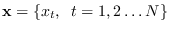 , be an autoregressive process (AR) of order . This means
that
, be an autoregressive process (AR) of order . This means
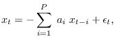
that  is obtained from the recursion
 |
(10.39) |
where
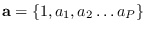 are the AR coefficients, and
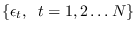 are independent, identically distributed
Gaussian samples of mean zero and variance
are independent, identically distributed
Gaussian samples of mean zero and variance  , known as the
innovation process. Because such a linear expansion is called a regression
in the statistics literature, and is regressed on itself, it is known
as an autoregressive process. Note that
, known as the
innovation process. Because such a linear expansion is called a regression
in the statistics literature, and is regressed on itself, it is known
as an autoregressive process. Note that  is by definition unity so it carries no
information and we often leave it out of the discussion.
An AR process may also be viewed in terms of an infinite impulse-response
(IIR) filter operating on iid samples of Gaussian noise.
From systems theory, such a process may be represented by the linear system
is by definition unity so it carries no
information and we often leave it out of the discussion.
An AR process may also be viewed in terms of an infinite impulse-response
(IIR) filter operating on iid samples of Gaussian noise.
From systems theory, such a process may be represented by the linear system
In other words, is a process with Z-transform  produced by passing the innovations
process
produced by passing the innovations
process  through a linear filter with Z-transform
 where
where
The power spectrum of the AR process is (See eq. 10.8)
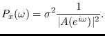 |
(10.40) |
The corresponding length- circularly-stationary process has circular
power spectrum (See eq. 10.9)
circularly-stationary process has circular
power spectrum (See eq. 10.9)
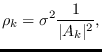 |
(10.41) |
Subsections
![$\displaystyle E(z) \rightarrow \left[ \frac{1}{A(z)} \right] \rightarrow X(z).
$](img1210.png)