For maximum entropy property,
the module designer must choose a reference
hypothesis and energy statistic
according to the requirements of Section 3.2.2.
Since  is positive valued,
energy statistics may be formed by
any weighted (with positive weights) sum of the samples of
is positive valued,
energy statistics may be formed by
any weighted (with positive weights) sum of the samples of
 |
(5.3) |
where  .
This class of energy statistic then has the properties
of a norm (See section 3.2.2)
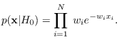
The canonical reference hypothesis corresponding to
this energy statistic is then
.
This class of energy statistic then has the properties
of a norm (See section 3.2.2)
The canonical reference hypothesis corresponding to
this energy statistic is then
Note that there is no reason to use another reference hypothesis
since all reference hypotheses that depend on the
data only through feature  will produce the same
resultant projected PDF [3].
The only difference lies in the tractability
of
will produce the same
resultant projected PDF [3].
The only difference lies in the tractability
of
 and for this class, we
provide a solution.
and for this class, we
provide a solution.
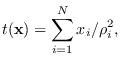
If the matrix A is already pre-defined,
one must determine an energy statistic that
is contained in (i.e. determine the weights
in (5.3).
For example, if matrix  implements the DCT, then
the first column is just a constant.
This suggests the energy statistic
implements the DCT, then
the first column is just a constant.
This suggests the energy statistic
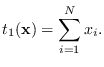
When in doubt and if matrix can be
modified, it may be reasonable to seek the
energy statistic that computes the total energy of the
source. Since generally comes from the magnitude-squared
output bins of an orthogonal transform, such as FFT,
it may be useful to use the energy statistic
which computes the total energy of the source
(input of the orthogonal transform).
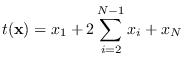
A special case of this is if matrix implements
the auto-correlation
function (ACF), then the statistic
is suggested (see Section 5.2.2).