It is possible to compute the PDF of  in the frequency domain. Let
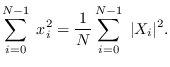
 be the DFT of . Note that
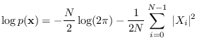
Therefore, for zero-mean Gaussian data with variance 1,
Although this is written in terms of  , it is a PDF of .
This distribution can be extended to arbitrary mean and power spectra, however we must be clear about
what we are assuming. Let  be defined as the
case when the DFT coefficients are independent zero-mean complex Gaussian RVs
and satisfy
be defined as the
case when the DFT coefficients are independent zero-mean complex Gaussian RVs
and satisfy
![$\displaystyle \rho_k = \frac{1}{N} \; {\cal E}\left\{ \vert X[k]\vert^2\right\}, \; 0\geq k < N,$](img1867.png) |
(17.4) |
where  are the power spectrum values. There are
  unique values of ,
being a symmetric sequence.
Note that the proper definition of power spectrum is through the Wiener-Kinchine theorem
in which the power spectrum is defined as the Fourier transform of the autocorrelation function.
In that case, the DFT of will neither exhibit independent
coefficients nor will the power spectrum be given by (17.4). These
relationships will only be approximate.
Hypothesis , however , is more useful to us when using finite-length
data samples and the DFT.
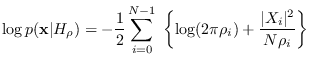
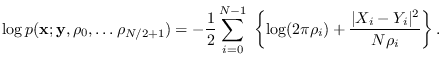
The PDF of under is precicely given by
unique values of ,
being a symmetric sequence.
Note that the proper definition of power spectrum is through the Wiener-Kinchine theorem
in which the power spectrum is defined as the Fourier transform of the autocorrelation function.
In that case, the DFT of will neither exhibit independent
coefficients nor will the power spectrum be given by (17.4). These
relationships will only be approximate.
Hypothesis , however , is more useful to us when using finite-length
data samples and the DFT.
The PDF of under is precicely given by
 |
(17.5) |
It is important to note that (17.5) is an exact PDF of under however
it is only an approximate PDF of for a stationary Gaussian process with power spectrum
 .
.
This is easily extended to an arbitrary mean.
Let
![${\cal E}({\bf x}) = {\bf y}= [y_1, \ldots y_N]^\prime$](img1871.png) be the mean of . Let
be the mean of . Let
 be the DFT of
  .
Then, consider the PDF
.
Then, consider the PDF
 |
(17.6) |
This is a useful and very tractable PDF.
Subsections