Computation of likelihood function using Proxy HMM

To implement (14.1), (14.2) brute-force is obviously impractical because of the combinatorial number of state sequences ${\bf q}$, but we can use the proxy HMM to do it efficiently. Note that each segmentation ${\bf q}$ corresponds to a distinct path through the proxy HMM state trellis, which has probability given by equation (14) in [65]. If we had the likelihood functions of each base-segment of the proxy HMM, the proxy likelihood function would be 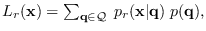$L_r({\bf x}) = \sum_{{\bf q}\in {\cal Q}} \; p_r({\bf x}\vert {\bf q}) \; p({\bf q}),$ where $r$ stands for “p(r)oxy", and where $\log p_r({\bf x}\vert {\bf q}) = \sum_{i=1}^T \; \log p({\bf x}^b_i \vert w_i({\bf q})),$ where ${\bf x}^b_i$ is the $i$-th base segment and $w_i({\bf q})$ is the proxy HMM state at time step $i$ corresponding to segmentation ${\bf q}$. The well-known HMM forward procedure [65] calculates the total proxy likelihood function $L_r({\bf x})$ efficiently using dynamic programming and without enumerating the segmentations.

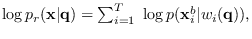
But the proxy log likelihood functions 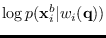$\log p({\bf x}^b_i \vert w_i({\bf q}))$ are defined for a single base segment, whereas the MR-HMM segment log-likelihood functions $\log p({\bf x}_s \vert m_s,k_s)$ are defined for segments spanning $k_s$ base segments. This problem is solved by writing $\log p({\bf x}_s \vert m_s,k_s)$ as a sum of $k_s$ equal parts: 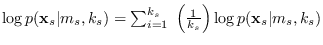$\log p({\bf x}_s \vert m_s,k_s) = \sum_{i=1}^{k_s} \; \left(\frac{1}{k_s}\right) \log p({\bf x}_s \vert m_s,k_s)$, where each part is assumed to apply to just one base segment, so can be used in place of the proxy segment log-likelihood functions. This substitution forces the proxy HMM forward procedure to compute $L({\bf x};$$\Lambda$$)$ for the the MR-HMM. This substitution can be more precicely written as

$$\log p({\bf x}^b_i \vert w_i({\bf q})) = (1/k_s) \; \log p({\bf x}_s \vert m_s,k_s),$$ (14.3)

where for segmentation ${\bf q}$, base segment time $i$ lies within segment $s$ of length $k_s$. The classical forward procedure applied to the proxy HMM then produces $L({\bf x};$$\Lambda$$)$. Furthermore, by calculating the backward procedure on the proxy HMM and combining with the forward procedure, we obtain the gamma probability $\gamma_i(m)$, which is the a posteriori probability that the system is in proxy state $m$ at base segment $i$ given all the available data. This is illustrated in Figure 14.1 as the filled-in circles in the proxy state trellis. These filled-in circles correspond to when $\gamma_i(m)$ has a high value. In the gap between the two pulses, is a case when probability is shared between more than one candidate path. If we sum up all the gamma probabilities for a given sub-class, we get an indication of the probability of each sub-class (illustrated at very bottom of Figure 14.1).