Proxy HMM

The proxy HMM is a hypothetical simple HMM that provides structure to the MR-HMM. It assumes that the input data is broken into small non-overlapping segments (called base segments) of $K$ samples. Let ${\bf x}^b_i, \;\;\; 1\leq i \leq T,$ be the base segments, where $T$ is the total number of base segments. We don't actually carve up the data into base segments - they are only used to understand the proxy HMM. Refer to Figure 14.1 , which illustrates the proxy HMM structure for $L=2$ sub-classes with designations “background" and “noise burst".

Figure 14.1: Illustration of the relationship between MR-HMM segmentation and proxy HMM trellis path.

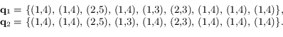
On the top is the time-series of length $T=34$ base segments wherein we see two bursts. Let the allowable segment sizes be $k\in\{1, \;\; 2, \;\; 3, \;\; 4, \;\; 5\}.$ Then, two possible segmentations ${\bf q}_1, {\bf q}_2$ for the time-series out of thousands of possible ones are , in format $(m,k)$, are:

$${\small \begin{array}{l} $ \mbox{\small ${\bf q}_1=$} \{(1,... ...5), (1,3), (1,4), (2,3), (1,4), (1,4), (1,4)\}.$ \end{array}}$$

These two segmentations are represented as dotted boxes drawn on top of the time-series and differ only in the way that the gap between the two bursts is divided, either as $(1,4), (1,3)$, or $(1,3), (1,4)$. We stress that these are just two of the many possible segmentations, all of which are considewred by the MR-HMM. In Figure 14.1 in the part labeled “Available Segments", we see all the allowable segment sizes and time shifts. The state trellis (“proxy state index" in figure 14.1) is divided into “partitions", each representing a choice of sub-class and segment size with vertical extent equal to the segment length. The paths corresponding to segmentations ${\bf q}_1$ and ${\bf q}_2$ are shown as dotted lines and filled-in circles, which are the proxy HMM states visited by the two candidate segmentations. The diagonal patterns are caused because once the system transitions into the first state of a partition, it is forced to complete the segment, counting out the states called wait-states. Note that all possible segmentations map to a unique path through the proxy HMM trellis. The proxy HMM parameters are created from the MR-HMM parameters $\Lambda$. The proxy state transition matrix (STM) is highly structured. The proxy has $N_p$ states consisting of all wait-states $N_p = \sum_{m=1}^L \; \sum_{i=1}^{n} \; k_i,$ ($N_p=25$ in Figure 14.1). The $N_p$ states are sub-divided into sub-classes and partitions, as explained above. The STM is sparse, mostly consisting of zeros and ones, which force the state to increment through the partition. Due to the forced wait-state counting, the proxy HMM has a very structured state transition matrix (STM). The proxy STM corresponding to Figure 14.1 is shown in Figure 14.2. Note the subdivision of proxy states into sub-class (solid lines) and partitions (dotted lines). The black circles indicate that once the system transitions to the start of a partition, it must increment to the end of the partition. The shaded circles indicate that the last wait-state of each partition may transition to the first wait-state of any partition. Since it involves a transition to a particular sub-class and segment size, the probability value is equal to the product of the sub-class transition probability ${\bf A}_{i,j}$ and the segment size probability $\rho_{m,i}$. The proxy initial state probabilities are conformal with any column of the STM, with values determined by the product of the of the sub-class initial probability $\pi_{i}$ and the segment size probability $\rho_{m,i}$.

Figure 14.2: The proxy STM corresponding to Figure 14.1. Empty circles are zero, black circles are 1.0 and shaded circles take a value between 0 and 1.