Multiple Records
It is fairly straight-forward to extend
the Baum-Welch algorithm to the case when
multiple observation sequences (“records") are available.
Rather than
 , we have
 .
For each record,
.
For each record,
- Run the forward-backward procedure on
 to produce
 ,
,
 ,
,
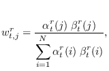
- Compute
 ,
,
 as in (13.14).
- Compute
 as in (13.15).
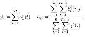
Then, we have
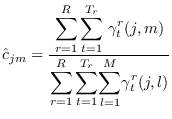
Updating the Gaussian mixture parameters
requires defining
which leads to
 through (13.20).
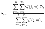
We then have
through (13.20).
We then have
and
... et cetera.