Reestimation of Gaussian Mixture Parameters

If $b_j(O)$ are modeled as Gaussian mixtures (GM), one could simply determine the weighted ML estimates of the GM parameters. Since only iterative methods are known, this would require iterating to convergence at each step. A more global approach is possible if the mixture component assignments are regarded as “missing data" [66]. The result is that the quantity

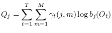$$Q_j = \sum_{t=1}^T \sum_{m=1}^M \gamma_t(j,m) \log b_j(O_t)$$ (13.19)

is maximized, where

$$\gamma_t(j,m) = w_{t,j} \left[ \frac{\displaystyle c_{jm} \; {\ca... ...c_{jk} \; {\cal N}({\bf O}_t,\mbox{\boldmath$\mu$}_{jk},{\bf U}_{jk}) } \right]$$ (13.20)

The weights $\gamma_t(j,m)$ are interpreted as the probability that the Markov chain is in state $j$ and the observation is from mixture component $m$ at time $t$. The resulting update equations for $c_{jm},$   $\mu$$_{jm}$, and ${\bf U}_{jm}$ are computed as follows:

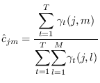$$\hat{c}_{jm} = \frac{\displaystyle {\displaystyle \sum_{t=1}^{T}}... ...e {\displaystyle \sum_{t=1}^{T}} {\displaystyle \sum_{l=1}^{M}} \gamma_t(j,l) }$$ (13.21)

Note the similarity to (13.2). This means that the algorithms designed for Gaussian mixtures are applicable for updating the state PDFs of the HMM.

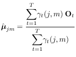$$\hat{\mbox{\boldmath$\mu$}}_{jm} = \frac{\displaystyle {\displays... ...,m) \; {\bf O}_t }{\displaystyle {\displaystyle \sum_{t=1}^{T}} \gamma_t(j,m) }$$ (13.22)

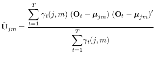$$\hat{{\bf U}}_{jm} = \frac{\displaystyle {\displaystyle \sum_{t=1... ...u$}_{jm})^\prime }{\displaystyle {\displaystyle \sum_{t=1}^{T}} \gamma_t(j,m) }$$ (13.23)

Note that the above equations do not treat the problem of constraining the GM covariances. This needs to be addressed (see section 13.2).