Derivation of the EM Algorithm for GM

Let ${\bf X}=\{{\bf x}_1, {\bf x}_2 \ldots {\bf x}_K\}$ be a collection of data. The Q-function is defined as the expected “complete" log-PDF where the expectation is carried out over the conditional distribution of the “missing data", given ${\bf X}$, using the current best estimate of the PDF parameters $\Lambda$, and the log-PDF is written in terms of the new values of the parameters to be estimated, $\Lambda^\prime$:

$$Q(\Lambda,\Lambda^\prime) \stackrel{\mbox{\tiny$\Delta$}}{=} {\r... ...p({\bf k}\vert {\bf X}; \Lambda) \log \; p({\bf X}, {\bf k}; \Lambda^\prime).$$

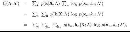
Expanding,

$$\begin{array}{rcl} Q(\Lambda,\Lambda^\prime) &=& \sum_{{\bf k}}... ... {\bf X}; \Lambda) \; \log \; p({\bf x}_n, k_n; \Lambda^\prime) , \end{array}$$

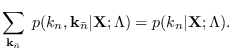
where ${\bf k}_{\bar{n}}$ are are the assignments not associated with sample $n$. The inner summation is a marginalization

$$\sum_{{\bf k}_{\bar{n}}} \; p(k_n, {\bf k}_{\bar{n}} \vert {\bf X}; \Lambda) = p(k_n \vert {\bf X}; \Lambda).$$

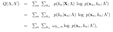
Thus,

$$\begin{array}{rcl} Q(\Lambda,\Lambda^\prime) &=& \sum_n \; \sum... ..._n} \; \omega_{k_n,n} \log \; p({\bf x}_n, k_n; \Lambda^\prime) , \end{array}$$

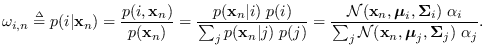
where the conditional model probabilities $\omega_{i,n}$ are defined as

$$\omega_{i,n} \stackrel{\mbox{\tiny$\Delta$}}{=}p(i \vert {\bf x}_... ...}({\bf x}_n, \mbox{\boldmath$\mu$}_j,\mbox{\boldmath$\Sigma$}_j) \; \alpha_j}.$$

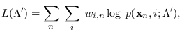
The maximization of $\Lambda^\prime$ can be carried out on the quantity

$$L(\Lambda^\prime) = \sum_n \; \sum_{i} \; \gamma_n \; \omega_{i,n} \log \; p({\bf x}_n, i; \Lambda^\prime) ,$$

where we have added data weights, $\gamma_n$, which define a probabilistic weights for each data sample. This could be interpreted as adjusting the influence of a training sample as though sample $n$ was replicated $\gamma_n$ times, or can be thought of as the probabilistic certainty that sample $n$ is indeed valid. By collecting $\gamma_n$ and $\omega_{i,n}$ together into a quantity $w_{i,n}$, we have

$$L(\Lambda^\prime) = \sum_n \; \sum_{i} \; w_{i,n} \log \; p({\bf x}_n, i; \Lambda^\prime) ,$$ (13.2)

where

$$w_{i,n} = \gamma_n\; \omega_{i,n}.$$

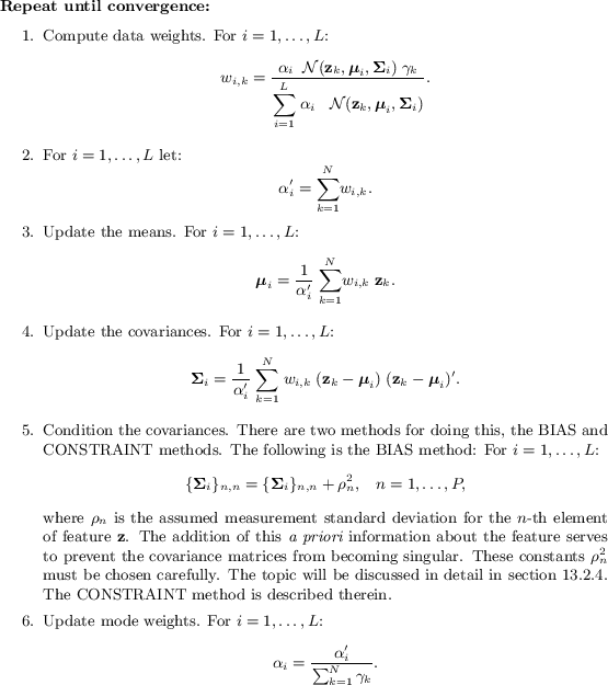
The algorithm in Table 13.1, maximizes (13.2) over $\Lambda^\prime$ at each iteration. While correct, it is representative only. Actual computation requires careful attention to numerical issues which are discussed below.

Table 13.1: Update Equations for Gaussian Mixtures. This is representative only. Actual implementation requires attention to numerical issues discussed in the text.