Implementation Overview

In the sections that follow, we discuss the subtleties associated with practical implementations of the E-M algorithm. We also discribe a complete MATLAB library for training, evaluating, and visualizing PDF's of high dimensions. The Gaussian mixture parameters are organized into a structure. The GPARM structure for feature dimension DIM with NMODES modes has the form shown in Table 13.2. To illustrate the use of the structure in MATLAB, if gparm is the name of the Gaussian mixture parameters, then the mixing weight of the third mode is accessed as gparm.modes(3).weight. A vector containing all the weights is created as follows: wts = [gparm.modes.weight]', whereupon wts is a NMODE-by-1 vector of mixing weights. The meaning of each parameter in the structure will be described.

Table 13.2: GPARM structure definition

The correspondence between the mathematical symbols and the MATLAB variables are tabulated in Table 13.3.

Table 13.3: Table of correspondence between MATLAB variables and mathematical symbols used in the text.

Parameter Name	Mathematical Symbol or Description
	$i\in[1\ldots L], \;\; n\in[1\ldots P]$
GM Parameters
DIM=length(gparm.features)	$P$
NMODES=length(gparm.modes)	Number of GM components, $L$
gparm.modes(i).weight	$\alpha_i$
gparm.modes(i).mean	$\mu$$_i$
gparm.modes(i).cholesky_covar	${\bf R}_i$
gparm.features(n).min_std	$\rho _n$
gparm.features(n).name	Feature Name
Other Variables
N	Number of input samples, $N$
data	Training data, ${\bf z}$
data_wts	Data weights $\gamma_k$

Some of these symbols are already defined. The rest will be defined later. The E-M algorithm of Table 13.1 is implemented by subroutine software/gmix_step.m. Training can be accomplished by calling software/gmix_step.m repeatedly. There are, however, subtleties having to do with how the GM is initialized and how the number of modes is chosen. Modes can be added or removed during the training process. The subtleties are described in the following sections. In the software, the subroutine software/gmix_trainscript.m handles the details. A simplified version software/gmix_est.m is good for general purose PDF estimation if you know how many modes to use.

To illustrate the PDF estimation problem, we will use some 3-dimensional features from a mysterious source. Samples of the feature vector ${\bf z}=\{z_1, z_2, z_3\}$ were used as training data and were stored in variable data1, which is of size 3 by $K$, where $K$ is the number of independent samples. Each row of the matrix stores the samples of a different feature. The following code segment implements the training and displays the resulting PDF in a density plot.

        NMODE=10;
        min_std = [20 20 1.0];
        names = {'Z1','Z2','Z3'};

        gparm1 = init_gmix(data1,NMODE,names,min_std);
        for i=1:100,
           [gparm1,Q] = gmix_step(gparm1,data1);
           fprintf('%d: Total log-likelihood=%g\n',i,Q);
        end;
        gmix_view2(gparm1,data1,1,2);

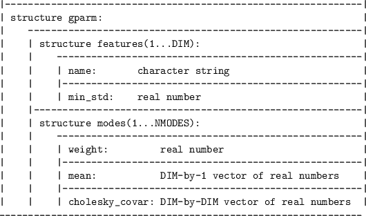
Refer to table 13.3 for symbol names. The variable names is a cell array that stores the feature names for use in visualization plots. The variable min_std stores the minimum feature standard deviations (See section 13.2.4). The routine software/init_gmix.m creates an initial set of parameters. In simple problems, the mixture can be trained by repeated calls to software/gmix_step.mas shown. In more difficult problems, it is necessary to do more to insure that there are the right number of modes and that the algorithm is converging properly. A representative MATLAB program for training are software/gmix_est.m and software/gmix_trainscript.m, which in turn call software/gmix_step.m, the subroutine that actually implements the E-M algorithm. We will discuss the use of software/gmix_trainscript.m and software/gmix_est.m in more detail in the following sections. Results of running the above code segment are shown in Figure 13.1.

Figure: Results of PDF estimation for the 3-dimensional feature vector ${\bf z}=\{z_1, z_2, z_3\}$. Data and PDF's are projected on the ($z_1,z_2$) plane. The three cases are for 12, 100, and 500 training samples. The final number of mixture components ($L$) was 1, 6, and 8, respectively. The accuracy improves as the number of training samples increases.

Visualization is accomplished by software/gmix_view2.m for any desired 2-dimensional plane. A routine software/gmix_view1.mis also available for projecting on one axis using a histogram. We will describe a complete example in more detail in section 13.2.7.

Before iterating, a starting point is needed for the GM parameters. This is handled by software/init_gmix.m. This routine inputs some samples of data vectors ${\bf z}_1,\ldots,{\bf z}_N$, the number of GM terms to use ($L$), the covariance conditioning parameters $\rho _n$, and the names of all the features. The GM component means $\mu$$_i$ are initialized to randomly selected input data samples. The covariances are initialized to diagonal matrices with large variances. It is important to use variances on the order of the square of the data volume width $\vert\max(z)-\min(z)\vert^2$. The size of the variances at initialization determines the data “window" through which each GM component “sees" the data. Too small a window at initialization can lock the algorithm into the wrong local minimum of the likelihood function. The initial weights $\alpha_i$ are set to be all equal.

There are two approaches to determining the number of modes. The first is to sprinkle a large number of modes throughout the data volume and remove the weak or redundant ones as it converges. The second approach is to start with just one mode and add modes as needed. The way you determine if a new mode is needed (by splitting an existing mode) is by a skew or kurtosis measure (software/gmix_kurt.m). These two methods, called top-down and bottom-up, respectively will be covered in section 13.2.5.