An Example Script for Gaussian Mixtures

Script software/gmix_example.m is designed as a teaching example for use of the software. All the basic functions as well as some handy utilities are demonstrated. Refer to the program listing for the discussion that follows. After typing » gmix_example at the MATLAB prompt, you will see the graph of Figure 13.11 and the program will pause.

Figure 13.11: Samples from a Gaussian mixture.

This is a two-dimensional “point scatter" diagram of the data that we will fit a Gaussian Mixture to. Refer to the program listing to see how this data is created. Pressing any key initializes the Gaussian Mixture parameters with the following 3 lines:

   names={'ENGY','TIME'};
   min_std = [.1 .1];
   NMODE=1;
   gparm1=init_gmix(data1,NMODE,names,min_std);

The first line assigns names to the two dimensions. We have chosen to call them "ENGY" and "TIME". The next line assigns the $\rho _n$ parameters, as discussed in section 13.2.4. The $N$ training data samples are stored in the $P\times N$ variable data1. The last line creates the parameter structure gparm1. Since the algorithm starts with just a single mode (NMODE=1), the approximation is poor (Figure 13.12).

Figure 13.12: The initial Gaussian mixture approximation.

Pressing a key again executes the training with a 150-iteration limit:

	gparm1=gmix_trainscript(gparm1,data1,150);

The log likelihood (Q) is printed out at each iteration along with the number of modes. Log likelihood would monotonically increase, if not for the pruning, splitting, and merging operations. Use of the CONSTRAINT method of covariance conditioning will also affect the monotonicity. It may be verified, however, that calls to software/gmix_step.m with BIAS=1 will result in monotonic likelihood increase, with the possible exception of numerical errors at the very end of the convergence process. Whenever mode splitting occurs, the message “Adding a mode .." is printed. Whenever mode merging occurs, the message “Merging ..." is printed. Because in this example, we have initialized with just one mode, mode splitting is more likely that merging, although is is possible that after several modes have been split, they can be re-merged. This causes a “fight" between software/gmix_kurt.m which tries to split, and software/gmix_merge.m, which tries to merge. In software/gmix_trainscript.m, it is arranged to allow time between splitting and merging so that the E-M algorithm can settle out. Otherwise, newly merged modes could be quickly split, or newly split modes could be quickly merged.

Once software/gmix_trainscript.m converges, you should should see the graph on the left of Figure 13.13.

Figure 13.13: Gaussian mixture approximation after convergence.

These plots are produced by software/gmix_view2.m. This utility is perhaps the most useful visualization tool for high-dimensional PDF estimation. It allows the data scatter plot to be compared with the marginalized PDF on any 2-dimensional plane.

Marginalization is a simple matter for Gaussian mixtures. Let ${\bf z}= [z_1, z_2, z_3, z_4]$. To visualize on the $(z_2,z_4)$ plane, for example, we would need to compute

$$p(z_2,z_4) = \int_{z_1}\int_{z_3} p(z_1,z_2,z_3,z_4) d z_1 dz_3.$$

Instead of integrating out $z_1, z_3$, marginalization requires only stripping out the first and third elements of each mode mean vector, and the first and third rows and columns of each mode covariance, then computing the resulting Gaussian mixture! Because we work with the Cholesky decomposition of the mode covariances, it requires stripping out the necessary columns, then doing a QR decomposition of the result. This stripping operation is performed by software/gmix_strip.m. The syntax would be:

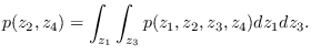
	gparm_out = gmix_strip(gparm_in, [2 4]);

where the second argument indicates that we want to retain the second and fourth dimensions. Using this method, the marginal distribution of any 2-dimensional plane is easily computed. Stripping is handled automatically by software/gmix_view2.m.

Press once more and the intensity plot is replaced by a contour plot of the modes (on the right of Figure 13.13. The contour plot is obtained by the fourth argument to software/gmix_view2.m. The complete syntax of software/gmix_view2.m is

	[p,xp,yp]=gmix_view2(gparm1,data1,idx1,idx2,[do_ellip],[M],iplot);

where idx1, idx2 are the indexes of the dimensions requested and do_ellip is an optional argument that, if equal to 1 (default=0), produces a contour plot of each mode instead of an image. M is an optional parameter that defines the number of resolution cells for each dimension of the plot (default=60). The optional parameter iplot can be set to zero if only the outputs p,xp,yp are wanted. These outputs provide the output PDF grid that can be plotted by imagesc(xp,yp,p). In the example, since the data is 2-dimensional to begin with, there is no dimension reduction performed by software/gmix_view2.m.

Information about the Gaussian mixture may be printed by calling software/gmix_show.m. This information, which includes the mode weights, means, and determinants, can be directly compared with Figure 13.13. The true means are (2,3) and (.5,.5), and the true determinants are 1.44 and 1.0, respectively. Generally, if the algorithm results in just 2 modes, the parameters agree very closely. The inclusion of a third or fourth mode makes it difficult to see the correspondence. But, nevertheless, the PDF approximation is good as evidenced by the intensity plot. You can run software/gmix_example.m again and each time the result will be a little different. But always, the intensity plot and the PDF approximation is excellent.

Press the key once more and Figure 13.14 will be plotted.

Figure 13.14: One dimensional PDF plots; Marginal PDF's compared to histograms.

This figure shows the 1-dimensional marginals for each dimension displayed along with the histograms. It is the result of calling software/gmix_view1.m. The calling syntax is

	[pdf,xp,h,xh]=gmix_view1(gparm,data,idx,nbins);

If called without any output arguments, the plot will automatically be generated. Input idx is an array of indexes for the dimensions desired. For more than one index, multiple plots are produced. Input “nbins" is the histogram size.

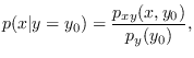
Press a key once more and Figure 13.15. This figure demonstrates the function gmix_cond (See Section 13.2.6) which creates conditional PDFs from the original Gaussian mixture. Rather than using Bayes rule explicitly to compute the conditional PDF of x given that $y=y_0$,

$$p(x \vert y = y_0) = { p_{xy}(x,y_0) \over p_{y}(y_0) },$$

it solves for the Gaussian mixture parameters of $p(x \vert y = y_0)$ in closed form so that you can later evaluate $p(x \vert y = y_0)$ at any point $x$, or else examine the parameters of the mixture. The figure shows the PDF evaluated at four values of $y_0$.

Figure: Conditional PDFs of $x$ given $y=y_0$, at various values of $y_0$: {-1, 1, 3, 6} .

Press a key once more and Figure 13.16 is shown. This figure plots the original data again in green and some synthetic data created by software/gmix_makedata.m in red. This demonstrates a convenient aspect of GM approximation: generating synthetic data is simple.

Figure 13.16: Original data (green) and synthetic data (red).

Press a key once more and Figure 13.17 appears.

Figure 13.17: A second data class in yellow. The first data set in magenta.

We now have two data sets. We will now build a classifier using Gaussian mixtures. The first step is to train a second parameter set on the second data set. This time, we will use the top-down approach by initializing with 15 mixture modes. This time, there will be alot of merging and purging going on, but less splitting! Press a key again and the training starts. When complete, you should see Figure 13.18.

Figure 13.18: Result of top-down approach: Trained GM approximation of second class.

To classify, it is necessary to compute the log-likelihood of test data. This is done using software/lqr_evp.m. The name of the subroutine was not thought up logically, but evolved from (l)og-likelihood (ev)aluation from the (p)arameters, and the fact that the (QR) decomposition is involved in the covariance estimates! The calling syntax is

	loglik = lqr_evp(gparm1,data1,0);

If the third argument was 1, the routine would return a matrix of log-likelihoods where each column is from one of the mixture modes. The zero forces the modes to be combined with the apropriate weights into the GM approximation. The ROC curve is shown in Figure 13.19. Refer to the listing for details.

Figure 13.19: ROC curve for two-class problem.