Example of Estimation: Beam Interpolation

Assume that beam intensity values are available from a set of $M$ uniformly spaced (in direction) sonar or radar beams. A target exists somewhere in the span of the $M$ beams, yet we do not know its center location, nor do we know the width of the response to the signal (as in a broadband system with frequency-dependent beamwidth). We assume for simplicity that the amplitude is known, yet in principle, amplitude can be another unknown. Thus, there are two parameters we seek to estimate: direction $d$ and beamwidth $w$. This problem normally requires a search in the $d,w$ plane for best match (as in maximum likelihood). Using GM, we solve the problem without a search, yet achieve performance comparable to ML!

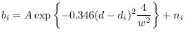
Let the beam pointing directions be $d_{1},\ldots,d_{M}$. Let the beam intensities ${\bf b}=\{b_{1}\ldots b_{M}\}$ be modeled by

$$b_{i} = A \exp\left\{ -0.346 (d-d_{i})^{2} \frac{4}{w^{2}}\right\} + n_{i}$$

where $n_{i}$ is a noise term (we use Gaussian noise in the simulation and CR bound analysis). This is a Gaussian beampattern with 3 dB width $w$.

A sample size of 4096 was created using $d$ and $w$ selected from uniform distributions in the ranges [-10,10], [15,50], respectively. Parameters were $A=50$, $\sigma^{2}=1$, $M=5$, $\{\theta_{i}\} = \{-20,-10,0,10,20\}$. A GM model $p({\bf b},d,w)$ of 12 modes was trained on the data. To illustrate the ability to create conditional distributions, $p(d,w\vert{\bf b})$ was computed for a sample of ${\bf b}$ computed for $d=2,w=18$ with no additive noise. The result appears in Figure 13.6. The visual effect of this figure is to say to the operator that there are no other values of interest except the peak.

Figure: Condition distibution of $d$ (THTA) and $w$ (WDTH) given a sample of ${\bf b}$ computed for $d=2,w=18$ with no additive noise.

It is also possible to condition on $d$ or $w$. The conditional distribution $p({\bf b},w \vert d)$ was computed for $d=0$ and $d= -5$. these plots are shown in Figures 13.7,13.8.

Figure: The condition distibution $p({\bf b},w \vert d)$ marginalized on each dimension of ${\bf b}$ for $d=0$.

Figure: The condition distibution $p({\bf b},w \vert d)$ marginalized on each dimension of ${\bf b}$ for $d= -5$.

Note that the beam output values have distributions symmetric about the value of $d$, as expected. Note also the wider spread of values on outer beams due to the variations in $w$.

Estimates of $d,w$ were obtained using formulas (13.8),(13.6). To determine bias, uncorrupted (no noise) values of ${\bf b}$ were created for a range of $d$ for $w$ fixed at 20, and for a range of $w$ for $d$ fixed at 2. These two graphs appear in Figures 13.9,13.10.

Figure: Plot of $\hat{d}-d$ for noise-free data with $w=20$.

Figure: Plot of $\hat{w}-w$ for noise-free data with $d=2$.

In each case, the bias error is plotted as a function of the variable parameter. Bias is clearly a function of the operating point. It is also a function of the number of modes and the convergence point of the GM approximation algorithm. Random error was determined by choosing a specific value of $d,w$ and running 300 trials with independent noise added to ${\bf b}$. The result of 300 trials is shown below.

	True Value	Mean	Variance	CR Bound
$d$	2	1.9435	.0550	.0493
$w$	18	18.003	.09756	.0945

Results of 300 trials, $A=50,\;\;\sigma^{2}=1, \: M=5.$

The results were in close agreement with the CR bound. Strictly speaking, the CR bound does not apply since the conditional mean estimator is biased for a fixed $d,w$ (it is unbiased for random $d,w$ conditioned on ${\bf b}$), however, the CR bound is useful for comparison purposes.