The GM representation of the density
has the a remarkable property that
 can
be computed in closed form.
This is especially useful in visualization of information.
For example, it is useful to show a human operator
the distribution of likely
can
be computed in closed form.
This is especially useful in visualization of information.
For example, it is useful to show a human operator
the distribution of likely  after
after  is
measured. If desired, the MMSE can be computed
in closed form as well. The MAP estimate can also be computed, but that
requires a search over .
is
measured. If desired, the MMSE can be computed
in closed form as well. The MAP estimate can also be computed, but that
requires a search over .
Let the GM approximation to the distribution be given by
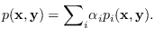 |
(13.4) |
By Bayes rule,
where
 is the marginal distribution
of . We now define
is the marginal distribution
of . We now define
 as the
marginal distributions of given that
is a member of mode
as the
marginal distributions of given that
is a member of mode  . These are,
of course, Gaussian with means and covariances
taken from the -partitions of
the mode mean and covariance
. These are,
of course, Gaussian with means and covariances
taken from the -partitions of
the mode mean and covariance

 .
.
Then,
 |
(13.5) |
where
 is the conditional
density for given assuming that and
are from that certain Gaussian sub-class .
Fortunately, there is a closed-form equation for
[63].
is Gaussian
with mean
is the conditional
density for given assuming that and
are from that certain Gaussian sub-class .
Fortunately, there is a closed-form equation for
[63].
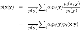
is Gaussian
with mean
and covariance
 |
(13.7) |
Note that the conditional distribution is a Gaussian
Mixture in its own right, with mode weights modified
by
which tends to “select" the modes
closest to . To reduce the number of modes
in the conditioning process,
one could easily remove those modes with a low value of
(suggested by R. L. Streit).
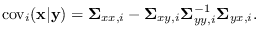
This conditional distribution can be used for data
visualization or, to easily calculate the
conditional mean estimate, which is a by-product
of equations
(13.5),(13.6),(13.7):
 |
(13.8) |
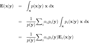
![$\displaystyle _{i} = \left[ \begin{array}{l}
\mbox{\boldmath$\mu$}_{x,i} \m...
...}_{xy,i} \\
{\bf\Sigma}_{yx,i} & {\bf\Sigma}_{yy,i} \\
\end{array} \right]
$](img1530.png)