MA Modeling

A moving average (MA) models is a special case of ARMA where $P=0$. An MA model assumes that the data $x_n$ is generated according to the recursion

$$x_n = \sum_{i=0}^Q \; b_i \; e_{n-i},$$ (10.36)

where $e_n$ are assumed to be $N(0,\sigma^2)$ iid RVs and $b_0=1$. Note that in MATLAB, an MA process can be generated with the filter command:

>> e=randn(N,1);
>> x=filter(b,1,e * sqrt(sig2));

which is directly equivalent to (10.36) except for the initial startup. To alleviate startup effects, it is necessary to discard the first $Q$ samples of x. In practice, one would generate $N+Q$ samples, then keep the last $N$ samples:

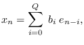
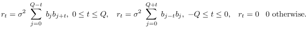
>> e=randn(N+Q,1);
>> x=filter(b,1,e * sqrt(sig2));
>> x=x(Q+1:Q+N);

In contrast to ARMA, MA has a finite ACF. An MA process has the autocorrelation function

$$r_t = \sigma^2 \; \sum_{j=0}^{Q-t} \; b_j b_{j+t}, \; 0 \leq t \l... ...; b_{j-t} b_{j}, \; -Q \leq t \leq 0, \;\;\; r_t=0 \;\;\; 0 \; {\rm otherwise}.$$ (10.37)

Note that $r_t$ is zero when $\vert t\vert>Q$. In MATLAB,

>> b2=conv(b(:),flipud(b(:)));
>> % Theoretical ACF of MA process
>> r = sig2 * [b2(1+Q:end); zeros(N-Q-1,1)];

The circular MA process is a special case of the circular ARMA process with PDF (10.7) and

$$\rho_k = \sigma^2 \; \vert B_k\vert^2.$$ (10.38)