Data PDF of circularly stationary process

For the circularly stationary process, equation (10.6) may also be used but the matrix ${\bf R}_N$ will not be Toeplitz, it will be circulant. A nice property of circulant matrices is that their eigenvectors are the DFT basis functions. As a result, (10.6) can be written in the discrete frequency-domain in terms of the circular power spectrum $\rho_k$:

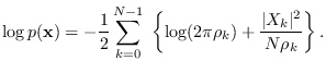$$\log p({\bf x}) = - \frac{1}{2} \sum_{k=0}^{N-1} \; \left\{ \log (2\pi \rho_k ) + \frac{\vert X_k\vert^2}{N \rho_k } \right\}.$$ (10.7)

Note well that although (10.7) is written in terms of $X_k$, it is a PDF of ${\bf x}$. It is only necessary to substitute (10.5) for $X_k$ to write the PDF in terms of ${\bf x}$. Then, when integrated over the $N$-dimensional space of ${\bf x}$, it gives 1. The circular stationary process has some very nice properties. It can be shown that the assumption of a circular stationary process means that the DFT coefficients $X_k$ are independent random variables. This has to do with the fact that the eigenvectors of the covariance matrix of ${\bf x}$, which is a circulant matrix, are the DFT basis vectors. An entire class of PDFs is created when an arbitrary positive function $\rho_k$ is used - the expression remains a PDF defined in ${\bf x}$ (See eq. 17.5). In other words, if we assume the DFT bins are independent and obey (10.4) for any function $\rho_k$, we obtain an exact and tractable expression for the PDF of a circularly stationary process ${\bf x}$ (See Eq. 17.5). This model can be used to approximate the PDF of any stationary process whose power spectrum is known.