Circularly-stationary process

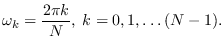
Equation (10.1) is of limited value in practice because it concerns infinite-length sequences and continuous-valued frequency. The theory of stationary processes can be adapted to finite-length time-records if we use the discrete Fourier transform in place of the Fourier transform. The concept of stationarity changes to circular-stationarity. Analogous to the Wiener-Kinchine theorem (10.1), the circular power spectrum is defined using the DFT pair

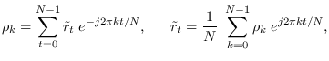$$\rho_k = \sum_{t= 0}^{N-1} \tilde{r}_t \; e^{-j2\pi k t/N}, \;\;\;\;\;\; \tilde{r}_t = {1\over N} \; \sum_{k= 0}^{N-1} \rho_k \; e^{j2\pi k t/N},$$ (10.2)

where $\tilde{r}_t$ is the circular ACF

$$r_k = \frac{1}{N} \sum_{i=1}^N \; x_i x_{[i+k]_N},$$ (10.3)

where $[i+k]_N$ means modulo-$N$.

For a periodic process $x_t$ that has a circular ACF, a circularly stationary process, the circular power spectrum is also defined by

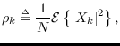$$\rho_k \stackrel{\mbox{\tiny$\Delta$}}{=}\frac{1}{N} {\cal E} \left\{ \vert X_k\vert^2 \right\},$$ (10.4)

where $X_k$ is the $N$-sample DFT of the length-$N$ sequence $x_t$,

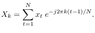$$X_k = \sum_{t=1}^{N} x_t \; e^{-j2\pi k (t-1)/N}.$$ (10.5)

Note that the circular power spectrum is the expected value of the magnitude-squared DFT bins and is defined only at the discrete DFT frequencies

$$\omega_k = \frac{2 \pi k}{N}, \; k=0, 1, \ldots (N-1).$$

Each stationary process can be approximated by a circularly stationary process whose circular power spectral values are the same as the power spectrum values of the stationary process. Unfortunately, if $P>0$, the ACF of the stationary process will be infinite in length because the output process has passed through an infinite impulse response (IIR) filter. So, the ACF, which is infinite, cannot be represented by the circular ACF. However, as long as the ACF of the original process dies to zero prior to lag $N/2$, the circular ACF will equal the original ACF over the first $N/2$ lags (See Figure 10.2). By using circularly stationary processes as approximations to stationary processes, we can obtain very efficient and tractable results for PDF analysis and feature design.