Next: Maximum Likelihood Parameter Estimation Up: Appendix Previous: Least Squares Contents
Proof:
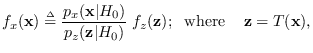
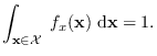
We show now that
![]() is a member of
is a member of
![]() .
.
Proof:
Let ![]() be drawn from the PDF
be drawn from the PDF
![]() and let
and let
![]() .
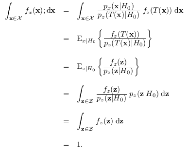
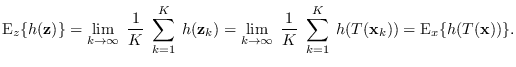
We now show that the PDF of
.
We now show that the PDF of ![]() is indeed
is indeed
![]() .
We prove this by showing that the moment generating function
(MGF) of
.
We prove this by showing that the moment generating function
(MGF) of ![]() is equal to the MGF corresponding to
is equal to the MGF corresponding to
![]() .
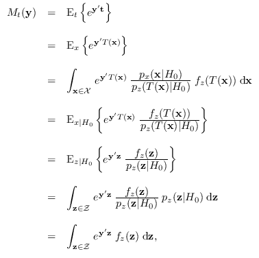
Let
.
Let
![]() be the joint moment generating function (MGF)
of
be the joint moment generating function (MGF)
of ![]() . By definition,
. By definition,
Another proof of the PPT is available [96].