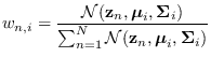
Splitting modes (gmix_kurt.m)
In a method proposed by N. Vlassis and A. Likas
[62], the number
of modes in a Gaussian mixture is determined by
monitoring the weighted kurtosis for each mode.
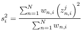
Putting their equation for one-dimensional  in our
notation, Vlassis et al define
in our
notation, Vlassis et al define
where
If
 is too high for any mode
  , they
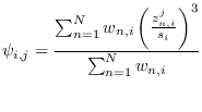
split the mode into two. We modify this for higher
dimension and use the skew in addition to the kurtosis.
Extending to higher dimension is
done by projecting each data
sample
, they
split the mode into two. We modify this for higher
dimension and use the skew in addition to the kurtosis.
Extending to higher dimension is
done by projecting each data
sample  onto the
  -th principal axis
of
-th principal axis
of

 in turn.
Let
in turn.
Let
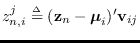 where
where
 is the -th column of
  , obtained
from the SVD of
(see discussion in section 13.2.5).
Thus, for each ,
, obtained
from the SVD of
(see discussion in section 13.2.5).
Thus, for each ,
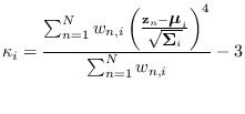
- Let
- Let
- Let
where
Now, if
 , for any , split mode .
Split the mode by creating modes at
, for any , split mode .
Split the mode by creating modes at
and
where  is the -th singular value of
. The same covariance
is used
for each new mode. Of course, the decision of whether to
split or not depends on the mixing proportion
is the -th singular value of
. The same covariance
is used
for each new mode. Of course, the decision of whether to
split or not depends on the mixing proportion
 as well. No splitting occurs
if is too small.
as well. No splitting occurs
if is too small.
In the following example, we create data with
a gap in it. We begin iterating with a single mode.
The kurtosis/skew algorithm above is able to assign modes until it
is finally happy after 8 modes (Figure 13.5).
Figure 13.5:
Results of bottom up PDF estimation.
One mode (left), two modes (center), and
after convergence at 8 modes (right).
|
|
The calling syntax for
software/gmix_kurt.m is
gparm = gmix_kurt(gparm,x,[kurt_thresh],[debug]);
The optional threshold parameter (default=1.0)
allows control over splitting. A higher
threshold is less likely to split.
The optional debug parameter, if set to 1, will print out
kurtosis and skew information.

![\includegraphics[width=2.1in,height=2.1in, clip]{ku1.eps}](img1518.png)
![\includegraphics[width=2.1in,height=2.1in, clip]{ku2.eps}](img1519.png)
![\includegraphics[width=2.1in,height=2.1in, clip]{ku8.eps}](img1520.png)