Merging Modes (gmix_merge.m)
Merging is creating a single mode from two
nearly identical ones.
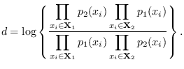
The closeness of two modes is determined
by
software/mode_dist.m which works as follows.
Let there be two PDF's  and
and  . Let there
be a collection of points
denoted
. Let there
be a collection of points
denoted
 near the central peak of
and a collection of points
denoted
near the central peak of
and a collection of points
denoted
 near the central peak of
. Then we define the closeness metric
near the central peak of
. Then we define the closeness metric
Notice that this metric is zero when
 and less that zero when
 .
A threshold (usually about -1 * DIM) is used to determine if the modes are too close.
This threshold should increase (become more negative)
as the dimension goes up.
.
A threshold (usually about -1 * DIM) is used to determine if the modes are too close.
This threshold should increase (become more negative)
as the dimension goes up.
Since and are just two Gaussian modes,
it is easy to know where some good points
for  and
and  are. We choose the means (centers)
and then go one standard deviation in each direction
along all the principal axes. The principal axes
are found by SVD decomposition of
are. We choose the means (centers)
and then go one standard deviation in each direction
along all the principal axes. The principal axes
are found by SVD decomposition of
 (the Cholesky factor of the covariance matrix).
This is illustrated
in Figure 13.4 for a Gaussian mode of dimension
(the Cholesky factor of the covariance matrix).
This is illustrated
in Figure 13.4 for a Gaussian mode of dimension  .
There is a center point and two points per dimension.
Therefore there are
.
There is a center point and two points per dimension.
Therefore there are  points per mode,
and two modes, thus
points per mode,
and two modes, thus  points.
Figure:
The 5 summation points for a 2-dimensional mode.
Contour at 2 .
.
|
|
If two modes are found to be too close,
they are merged. Merging is forming a weighted sum of two modes
(weighted by
 ).
The new mean is thus
).
The new mean is thus
  |
(13.3) |
The proper way to form a weighted combination of the covariances is
not simply a weighed sum of the
covariances, which does not take into account
the separation of the means. You need to be
more clever. Consider the Cholesky
decomposition of the covariance matrix
 .
It is possible to consider the rows of
.
It is possible to consider the rows of
 to be samples of
  -dimensional vectors whose
covariance is
-dimensional vectors whose
covariance is
 , where is the dimension.
The sample covariance is,
of course
, where is the dimension.
The sample covariance is,
of course
 , Now, given two modes
to merge, we regard
, Now, given two modes
to merge, we regard
 and
and
 as two populations to be joined.
The sample covariance of
the collection of rows is the desired covariance.
But this assigns equal weight to the two
populations. To weight them by their respective weights,
we multiply them by
as two populations to be joined.
The sample covariance of
the collection of rows is the desired covariance.
But this assigns equal weight to the two
populations. To weight them by their respective weights,
we multiply them by
 and
and
 .
Before they can be joined, however, they must
be shifted so they are re-referenced to
the new central mean. Here is a summary of the method:
.
Before they can be joined, however, they must
be shifted so they are re-referenced to
the new central mean. Here is a summary of the method:
- Let
 be as in (13.3).
- Let
 be the Cholesky factor of
 ,
,  .
.
- Let
 , each
  .
.
- Add the vector
 to each row of
  ,
each .
,
each .
- Multiply by
 , each .
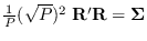
- Form
- Then the new covariance is
 , or
take the QR-decomposition of
, or
take the QR-decomposition of
 as the
Cholesky factor of the new covariance.
as the
Cholesky factor of the new covariance.
The above algorithm is implemented by
software/merge.m.
The subroutine that iterates over all the pairs of modes
and calls
software/merge.m and
software/mode_dist.mis
software/gmix_merge.m.
The calling syntax for
software/gmix_merge.m is
gparm = gmix_merge(gparm,max_closeness)
A good choice for the max_closeness threshold
is about -1.0 times , the PDF dimension.
![$\displaystyle {\bf C}=\left[
\begin{array}{c} {\bf C}_1 \cdots {\bf C}_2
\end{array}\right]
$](img1499.png)
![\includegraphics[scale=0.6, clip]{closest.eps}](img1484.png)