Data Re-synthesis

The estimation of the AR and sinusoid parameters is an iterative feature extraction approach. Despite this, given a set of estimated or randomly-selected parameters, we can create data that has the prescribed ML parameter estimates. We use the approach of Section 4.6.4 and 4.4.

Given a set of SINAR parameters, we first un-do the SNR norlalization, which was described in Section 9.2.1. Then, we can construct the the vector ${\bf y}$ and matrices ${\bf W}, {\bf H}, {\bf A}$, then using (9.15), we can require ${\bf x}$ to meet the condition

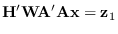$${\bf H}^\prime {\bf W} {\bf A}^\prime {\bf A} {\bf x}= {\bf z}_1$$ (9.18)

where

$${\bf z}_1 = \left( {\bf H}^\prime {\bf W} {\bf A}^\prime {\bf A} {\bf W} {\bf H}\right) {\bf b}.$$

Then, using the fact that the derivative w/r to frequency must be zero and using (9.14), we can also require that ${\bf x}$ meet the condition

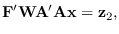$${\bf F}^\prime {\bf W} {\bf A}^\prime {\bf A} {\bf x}= {\bf z}_2,$$ (9.19)

where

$${\bf z}_2 = {\bf F} ^\prime {\bf W} {\bf A}^\prime {\bf A} {\bf y}.$$

Any generated data ${\bf x}$ must therefore meet the two linear constraints (9.18), (9.19). These two constraints insure that the ML sinusoidal parameter estimates will coincide with the desired ones and can be written as one linear constraints by stacking the matrices.

The constraints can be also implemented in the “whitened" domain. That is to say that the whitened data

$$\tilde{{\bf x}}={\bf A}{\bf x}$$

must meet the modified constraints

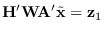$${\bf H}^\prime {\bf W} {\bf A}^\prime \tilde{{\bf x}} = {\bf z}_1$$ (9.20)

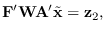$${\bf F}^\prime {\bf W} {\bf A}^\prime \tilde{{\bf x}} = {\bf z}_2,$$ (9.21)

We stack the matrices to produce the single constraint

$$\tilde{\bf C}^\prime \tilde{{\bf x}} = {\bf z},$$

where

$$\tilde{\bf C}= \left[ {\bf A} {\bf W} {\bf H}, \; {\bf A} {\bf W}... ... {\bf z} = \left[ \begin{array}{l} {\bf z}_1 \\ {\bf z}_2 \end{array}\right].$$

Now, in order to approximately meet the AR constraints, the whitened residual $\tilde{\bf e}=\tilde{\bf x}-\tilde{\bf y}$, where $\tilde{\bf y} = {\bf A} {\bf y},$ must have variance $\sigma^2$. Now $\tilde{{\bf x}}$ must meet $\tilde{\bf C}\tilde{{\bf x}} = {\bf z}$ as well as the constraint

$$\left(\tilde{\bf x}-\tilde{\bf y}\right)^\prime \left(\tilde{\bf x}-\tilde{\bf y}\right) = N \sigma^2,$$

which can be written

$$\tilde{\bf x}^\prime \tilde{\bf x} = z_0,$$

where

$$z_0 = N \sigma^2 +2 {\bf z}_1^\prime {\bf b} -\tilde{\bf y}^\prime\tilde{\bf y}.$$

To generate data that meets these constraints, we we follow the approach of Section 4.6.4. To generate this data, let

$$\tilde{{\bf x}}=\tilde{{\bf x}}_0 + \tilde{\bf C}^\perp {\bf u},$$

where $\tilde{\bf C}^\perp$ is the ortho-normal matrix of basis functions that span the orthogonal complement of $\tilde{\bf C}$. Since $\tilde{\bf C}$ is of dimension $N\times 3k$, then $\tilde{\bf C}^\perp$ is of dimension $N\times (N-3k)$. To meet $\tilde{\bf x}^\prime \tilde{\bf x} = z_0,$ we need vector ${\bf u}$ to have norm

$$\sqrt{{\bf u}^\prime {\bf u}} = \sqrt{z_0-\tilde{{\bf x}}_0^\prime \tilde{{\bf x}}_0}.$$

So, to create data $\tilde{{\bf x}}$, generate an $(N-3k)\times 1$ vector ${\bf u}$ of independent Gaussian noise, then normalize it to have norm $\sqrt{z_0-\tilde{{\bf x}}_0^\prime \tilde{{\bf x}}_0}$, then let $\tilde{{\bf x}}=\tilde{{\bf x}}_0 + {\bf C}^\perp {\bf u}.$ This vector will meet conditions ${\bf C}^\prime {\bf x}= {\bf z}$ as well as $\left(\tilde{\bf x}-\tilde{\bf y}\right)^\prime \left(\tilde{\bf x}-\tilde{\bf y}\right) = N \sigma^2.$

If we un-whiten $\tilde{{\bf x}}$ as follows:

$${\bf x}= {\bf A}^{-1} \tilde{{\bf x}},$$

which can be achieved in the frequency domain by dividing each Fourier coefficient by $A_k$, we will have an approximate solution to re-synthesis. But, although ${\bf x}$ meets the linear constraints exactly (for amplitude and derivative), it does not meet the auto-correlation function (ACF) constraints. We must insure that ACF computed from the residual ${\bf e} = {\bf x}-{\bf y}$ satisfies the desired ACF, which is the ACF of the autoregressive spectrum $r_t = {\rm IFFT}\left( {\sigma^2 \over \vert A_k\vert^2}\right),$ for $t=0,1 \ldots P$. This can be achieved by making a slight adjustment to ${\bf x}$ within the linear subspace orthogonal to the already-satisfied linear constraints. The linear constraints (in the un-whitened world) are given by

$${\bf C}^\prime {\bf x}= {\bf z},$$

where

$${\bf C}= \left[ {\bf A}^\prime {\bf A} {\bf W} {\bf H} , \; {\bf A}^\prime {\bf A} {\bf W} {\bf F}\right],$$

Let matrix ${\bf C}^\perp$ be the ortho-normal matrix spanning orthogonal complement space of matrix ${\bf C}$. Then, if we let ${\bf x}= {\bf y}+ {\bf C}^\perp {\bf v}$, and select ${\bf v}$ to meet the above circular ACF constraints, we have a solution that meets all constraints. This re-synthesis technique is implemented in software/module_sinar_synth.m.