Let's assume there are  tonals in
AR noise of order
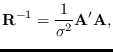
tonals in
AR noise of order  . There are
  parameters for each tonal:
frequency, amplitide and phase, or equivalently
frequency and complex amplitude with two
components (in-phase and quadrature), then the
parameters for each tonal:
frequency, amplitide and phase, or equivalently
frequency and complex amplitude with two
components (in-phase and quadrature), then the  AR parameters for a grand total of
 parameters.
Let the data be written
parameters.
Let the data be written
where  ranges from
  to
to  ,
,
 is auto-regressive noise and
is the deterministic (tonal) component,
and
and  are the time-series window function
coefficients (Hanning, etc.).
are the time-series window function
coefficients (Hanning, etc.).
In a more compact matrix notation,
we let
where  is the diagonal matrix of window function
coefficients.
is the diagonal matrix of window function
coefficients.
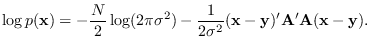
The log-likelihood function is given by
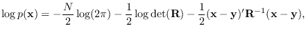 |
(9.11) |
where  is the auto-correlation matrix
for an AR process (see Section 10.1.3).
is the auto-correlation matrix
for an AR process (see Section 10.1.3).
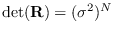
We break down
 into its
well-known Cholesky factor form
into its
well-known Cholesky factor form
where  is the prewhitening matrix, which is a
banded matrix formed from the prediction error filter.
Each row of is formed from the
prediction error filter
is the prewhitening matrix, which is a
banded matrix formed from the prediction error filter.
Each row of is formed from the
prediction error filter
![${\bf a}=[0, 0, \ldots, 0, a_P, \ldots, a_2, a_1, 1,
0, \ldots 0]$](img988.png) , where the occupies the main diagonal.
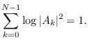
Matrix has a determinant of 1, as it is lower-triangular
and has ones on the diagonal.
For the non-circular (stationary process) case,
on the rows less than row , the prediction error filter
is truncated, and so the coefficients
must be estimated from the corrsponding lower-order AR model.
We can avoid the complexities of these end effects, especially
since we are assuming that a window function
is applied to the data, by assuming a circular
AR process (See sections 10.1.2, 10.2.4).
Then, matrix is circulant, with each row containing
the full prediction error filter, wrapped around.
Furthermore, the equation
, where the occupies the main diagonal.
Matrix has a determinant of 1, as it is lower-triangular
and has ones on the diagonal.
For the non-circular (stationary process) case,
on the rows less than row , the prediction error filter
is truncated, and so the coefficients
must be estimated from the corrsponding lower-order AR model.
We can avoid the complexities of these end effects, especially
since we are assuming that a window function
is applied to the data, by assuming a circular
AR process (See sections 10.1.2, 10.2.4).
Then, matrix is circulant, with each row containing
the full prediction error filter, wrapped around.
Furthermore, the equation
 holds exactly. We can therefore re-write (9.11) as:
 |
(9.12) |
The frequency-domain equivalent of (9.12)
is
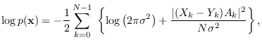 |
(9.13) |
where  and
and  are the Fourier coefficients of
 and
and  , respectively.
In obtaining (9.13), we used the fact that
, respectively.
In obtaining (9.13), we used the fact that
This is just the frequency-domain equivalent of saying that the
determinant of the circulant matric , with all ones on the
diagonal, is 1.
Although written in terms
of Fourier coefficients, the expression is a PDF of .
The equivalence of (9.13) and (9.12)
can be readily seen.
Subsections
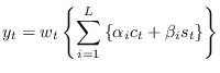
![$\displaystyle {\bf H} =
\left[ \begin{array}{llllllll}
c_{1,1} & c_{1,2} & \cdo...
...} \\
\beta_{1} \\
\beta_{2} \\
\vdots \\
\beta_{L} \\
\end{array} \right],$](img982.png)